We released our first version of Flaneer in mid-March 2021.
Since then, we have conducted several tests with small entities, such as Game Development or Post-production Studios and signed several clients.
We also launched a test with a French engineering University: MINES Paristech - PSL.
While this test took place 9 month ago, we believe this is an amazing example to show for a few reasons:
It showcases how students and teachers can work and collaborate together remotely, without investing in expansive laptops,
A good user experience is everything: students worked much more in a simple, ready to use and powerful environment,
By using heavy software and GPUs in the cloud, we show how students, but more generally, engineers, can work and reduce their IT costs,
The goal was simple: give access to engineering software (Fusion360, Abaqus, 3DExperience, Paraview, internal tools & python scripts) with the computing power needed (32GB RAM & a GPU per student) everywhere.
Given the sanitary context in Paris at the time, this last point was crucial: students had to work even if the school was closed.
The mission of each students group was to build a drone, from its conception to making it fly!
The solution we provided was for each student to remotely access a Virtual Machine running on Windows via a streaming protocol. Software were already installed, and files & folders were managed with our custom file system management.
While each beta test so far was a success, we use the example of MINES Paristech - PSL to dive deep into the usage & feedbacks of each student, mainly because this is the first one that was conducted at length (from March 24 to April 28) and at scale (~100 students & teachers).
Usage
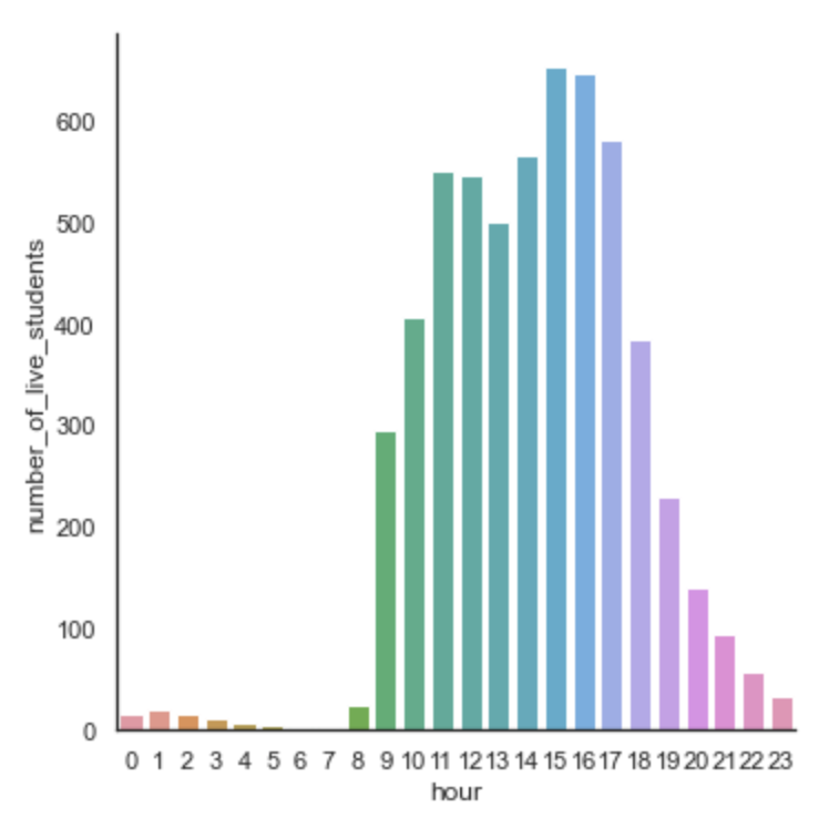
First, let’s have a look at the raw numbers. Students launched 1584 streaming sessions, each of them lasting 3.2 hours on average. Overall, students used Flaneer for more than 5000 hours, with around 10% of the usage during the weekend. Even if the students’ official hours were from 9 am to 5 pm, we still record many sessions outside of this time range.
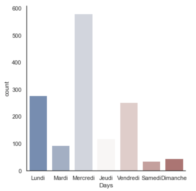
A large portion of the sessions took place on Wednesday & Monday when working with professors or tutored. However, on Friday (personal project time) or during the rest of the week (even weekends), we can observe a lot of sessions being streamed. (40% of them!)
It shows that a tool like Flaneer allows students to work more freely and when they need to (or where they need to).
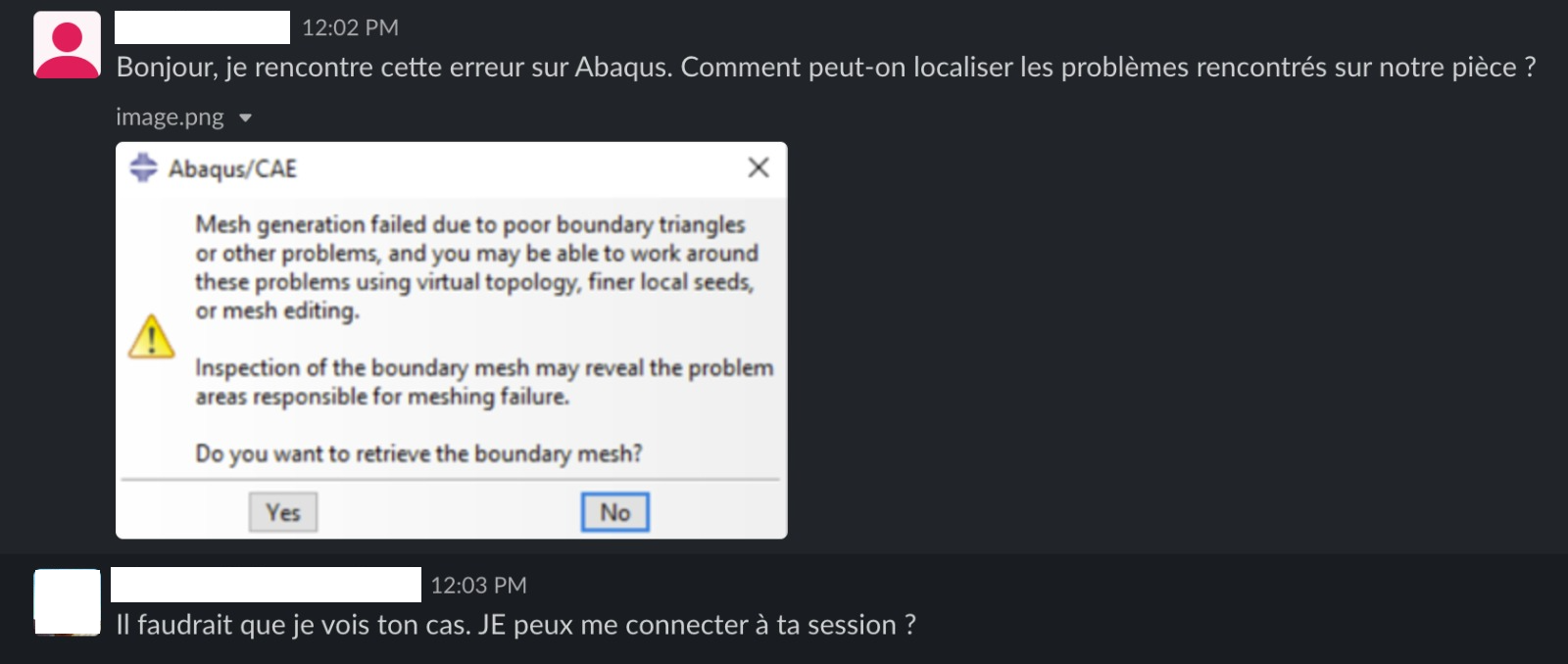
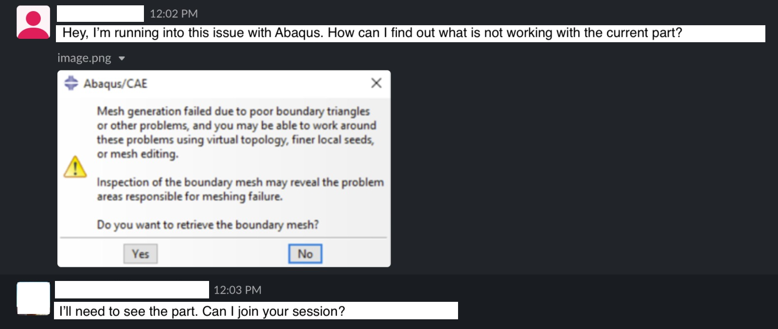
We believe Flaneer is the right tool to allow collaboration between students or between a student & a teacher. In our case, one can join the session of someone else & start working with him directly. Even more, if a student gets stuck using software, someone can immediately help him no matter where he is.
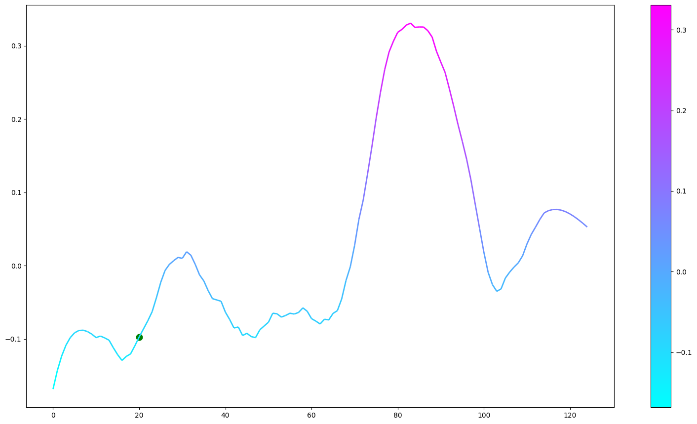
We counted 229 requests to join the session of another person, aka. 229 times where Flaneer helped two people work together.
Number of invocation of the “join another session” function
We strongly believe that sharing a session, and software per se, is the right way to collaborate. This solves hundreds of use cases, especially in a hybrid era when more & more will want to work from wherever they want.
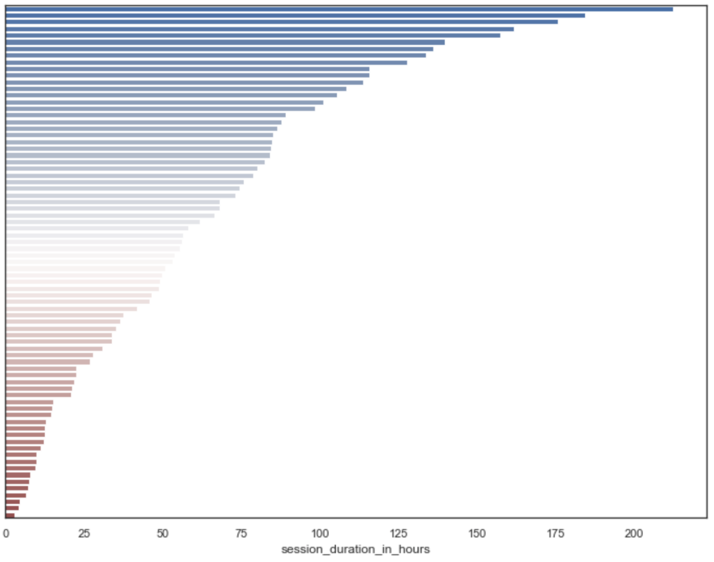
One could ask if Flaneer was used by the entire batch of students or not; let’s dive into that matter. We launched sessions for 77 distinct students, each launching between 1 & 55 sessions, streaming between 3 & 212 (!) hours. On average, students used Flaneer for 61 hours, launching on average 19 sessions
75% of the students used Flaneer for more than 20 hours
90% of the students used Flaneer for more than 10 hours.
25% of the students spent more than 85 hours on Flaneer!
Bugs & Reports
We used a slack channel & a live chat on our web app to talk directly with teachers & students. Everyone at Flaneer is a firm believer in self-onboarding & direct customer relations.
That means that using Flaneer should be as simple as it can get and that whenever something is not going according to plan, anyone can directly talk to use and get an answer (yes, that’s even true at 3 in the morning - we have pretty loud alarms & slack bots).
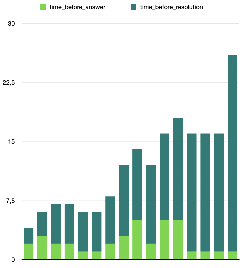
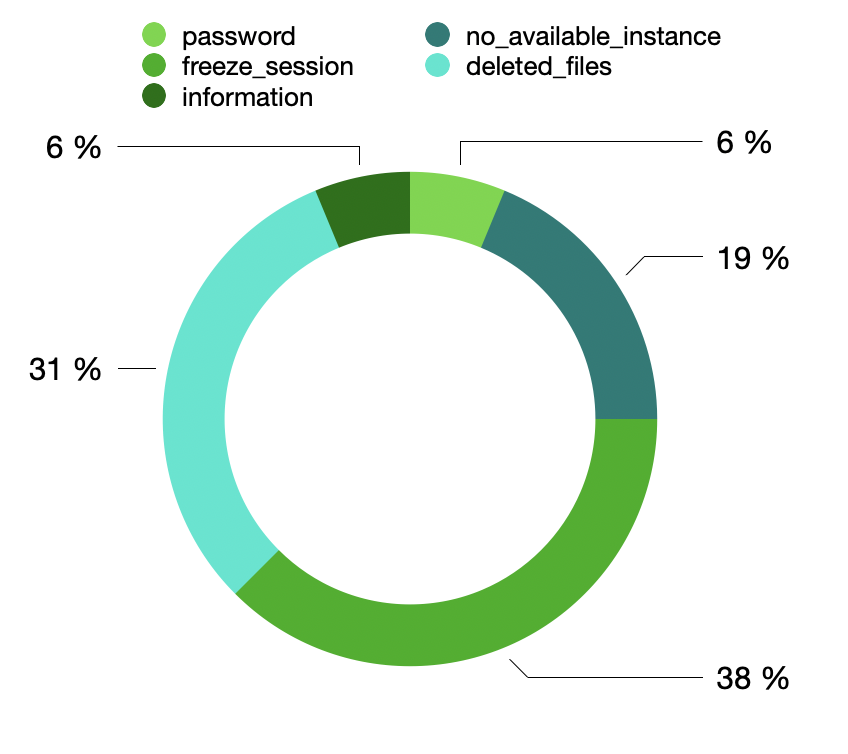
Most of the requests were solved in under 5 minutes, but we present here the requests that took above 5 minutes to get resolved or answered:
Only one issue took more than 20 minutes to get solved (we found a significant bug with the reset_password function that time). The other issues are available below:
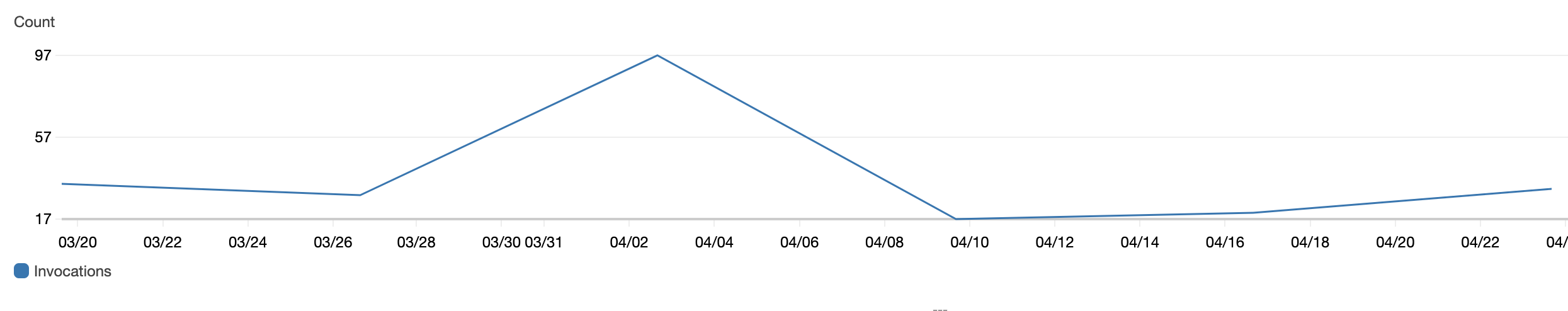
→ No sessions were available: the student had to wait for ~10/15 minutes before a new one was available. This did not happen very often. (cf image below)
→ The session freeze. This was easy to solve most of the time, simply by closing the browser tab & reopening it.
→ Some files were deleted from the student session. That is the most problematic bug we had.
Feedbacks
We received over fifty feedbacks from this beta test, and 95% of them were super positive. Regarding the overall quality of Flaneer:
50% of the students rated it a 5 out of 5
44% a 4 out of 5
6% a 1,2, or 3 out of 5.
We can also dive deeper into what the students liked & disliked. The most significant pain points we solved for the students are:
The file management system, allowing them to keep & store files outside of their computer
A life-saving solution when the laptop is a Chromebook or not good enough
Using software without downloading & managing them
How easy it was to use Flaneer
Being able to work anywhere & to switch computers seamlessly
Flaneer lets us achieve the type of teaching we want to do. We are not limited anymore by hardware or by long & complex talks with the IT department. Every teacher can now set up a workspace for their class in a matter of minutes. - Elie Hachem, Head of the Computing & Fluids Research Group @CEMEF - MINES Paristech
Now, we also have to look at what went wrong:
Some issues with the file management system, resulting in files being deleted for some users
Some latency issues
The streaming quality was sometimes too low (480p)
We were aware of some of these issues; we also believe that we still have a lot to work on regarding the sessions’ shortcuts while it did not come out. We were limited by streaming only in a browser, but the client version of our protocol now solves that!
We also worked closely with several professors working on this test and solved license server issues for them.
Conclusion
9 months later, we are still using the same recipe:
The simplest user experience we can provide
Software in the cloud, for everyone
Collaboration, no matter the tools or the software people are using
Providing support and feedbacks to our customers minutes or seconds after they need them
and are going for a lot more!
What’s your opinion about education & virtualization ? Feel free to comment or send me an email, I would love to have a chat with you!
Stay tuned for exciting Flaneer updates in the near future 🚀
You can also read more about us here: https://www.flaneer.com/blog/join-flaneer-engineering-team
Most of Flaneer services are hosted on AWS. That means that whether it is user data, files, or virtual workstation, it will be hosted on an AWS server. This article will dive into how we do it, how we make sure it is as secure as it can be, and how it will evolve over time.
Saying that everyone is concerned about their data and privacy seems obvious. At Flaneer, we’re working with multiple layers of sensitive data:
a company’s files system, such as Google Drive or One Drive
a team’s data and connection information
a user’s virtual workstation, aka its work, streaming over the internet
It is a necessity to build a safe and secure place for users to work.
The goals of this article are multiple. First, what is AWS and why do we consider it as a secure option? Then, how do we make it even safer? Finally, when will we switch to another cloud provider, especially a European one?
How do we work with AWS?
How do we work with AWS?
When you want to code something, be it a SaaS or a website, you will need to write code that will interact with a server. This server can store data or run some code. The critical part here is understanding where this particular server is and who is taking care of it. Most of the time, two solutions are possible (and being a startup working in infrastructure, trust me, it is not always an easy choice).
Solution 1: The company (here Flaneer, yours truly) will buy and manage its own hardware. This is a self-hosting solution.
Solution 2: The company (still Flaneer) will rent servers from someone else (a cloud provider). This is a cloud solution. While another company is renting you servers, they cannot access them. Only you are allowed to access and interact with them.
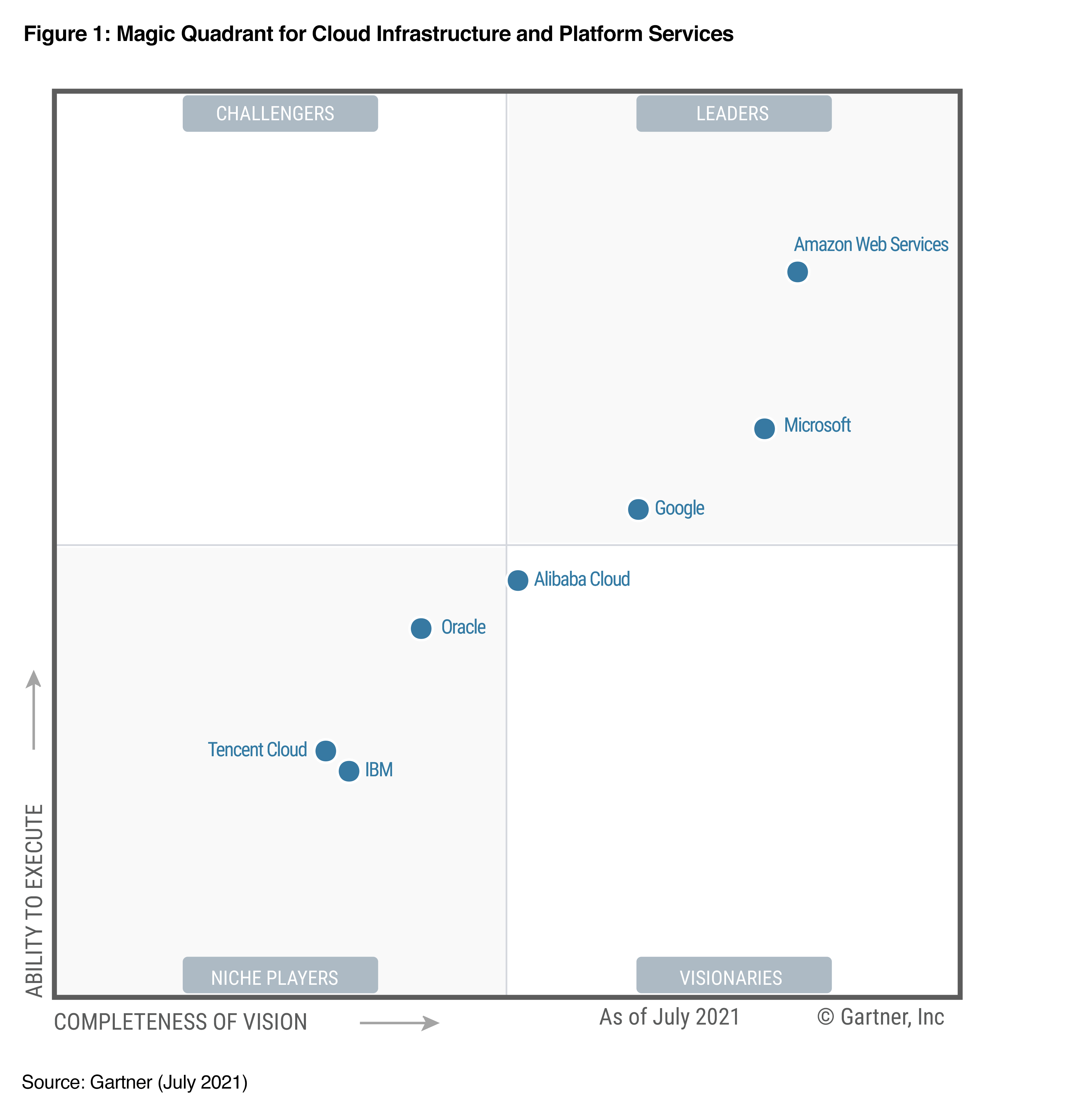
At this point, you probably guessed it: AWS was one of the possible cloud-provider we could go with. Other candidates are often:
GCP (Google Cloud Platform)
Azure (Microsoft)
and less often:
AliCloud (Alibaba)
Oracle
OVH
and even some very small and local ones. However, the smaller the provider, the less reliable and flexible it will be. It will also be much harder to scale up (or down, that happens sometimes).
This is why we went with AWS. It is the biggest cloud provider in the world and the one we felt the most comfortable to start with. Before diving into how we work with AWS, we think this might be a good time to answer some of the questions we often get asked while onboarding customers.
Why AWS and not another cloud provider?
AWS is probably the safest cloud provider out there. Security being our number one priority, it seemed like a no-brainer, and it still seems like it.
AWS is the most reliable cloud provider globally, with less than 2 hours of downtime per year. This is huge and can directly remove some cloud providers from the equation (looking at you OVH).
The amount of services AWS offers is massive. This allows our engineering team to quickly (that means less time than to make lunch — although that would depend on where you live and what you consider a good lunch (looking at my co-founder and his healthy Burger King habit here)) try and iterate on new solutions.
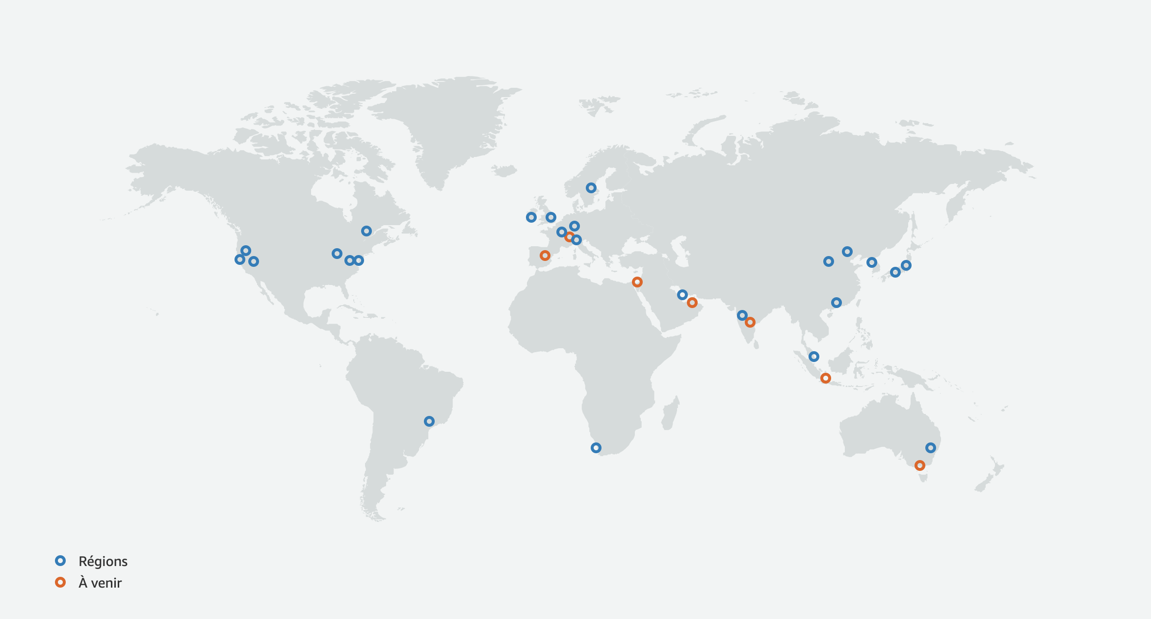
While not European, AWS has a lot of data centers in the world (cf Image 1). This allows us: 1. to easily use the closest servers to our customers; 2. to make sure these closest servers are actually close to the customer. On that note, since: Flaneer uses a French entity in Europe, and that most Flaneer users are European: this forces AWS to respect GDPR.
Why are we not self-hosting?
When you think about it, this makes a lot of sense, especially for a startup building a new infrastructure service from scratch. This would allow us to offer much lower prices and to customize much more the hardware we can offer.
However, this is extremely CapEx intensive and requires many skills that two recently graduated engineers did not have at the beginning. Messing with RaspberryPI, and building small clusters will not allow you to build massive infrastructure, trust me on that one.
However (trust our geeky side on that), we will work on that at some point during Flaneer’s life.
Why are my data safe & secure?
You can read extensively about why AWS is secure here: https://aws.amazon.com/security/?nc=sn&loc=0.
As an example:
AWS supports more security standards and compliance certifications than any other offering, including PCI-DSS, HIPAA/HITECH, FedRAMP, GDPR, FIPS 140–2, and NIST 800–171, helping satisfy compliance requirements for virtually every regulatory agency around the globe.
We talked a lot about how AWS is safe. But it is as safe as you make it. If you make a mistake, AWS will not save you: this is why we are extra cautious with every service we use. We’ll dive more into this subject in the next part.
What do we do with AWS?
At Flaneer, we use a lot (and by a lot, I mean it) of AWS services. We want to give a brief overview of the main ones and how they are related to our user’s data and privacy.
You can read more about how we use AWS and we make it as secure as possible here in
We are transforming IT Management to make it faster, simpler and accessible to everyone!
At Flaneer, we are building:
a new sort of computer that will change what software can do
an infrastructure capable of supporting our customers’ needs worldwide
tools to empower artists & workers around the world
We are trying to build an engineering team that reflects on these values: a simple and transparent infrastructure and development environment.
Being an engineer at Flaneer is simple. It means joining a small team of passionate engineers. Some of us worked at Amazon or Adore Me, others are open source contributors to large project such as Tor. But we all have one thing in common: we like to move fast, learn thing every day, and redefine software. We seek to maximise not only self productivity, but combined team productivity.
Does this sound like you?
Hungry and wants to change the way software are used — unstoppable with the right tools.
Bored and frustrated at big companies; feel held back by red tape, bureaucracy and poor decision making.
Consider yourself a generalist & enjoy being so: you are not tied down to a specific area, and are eager to learn new things every day.
Seeks to maximise not only self productivity, but combined team productivity, by communicating asynchronously.
Intellectually curious and loves learning.
We currently rent a private space at WeWork — Paris, but we mostly work remotely.
We are serious about competitive compensation and equity.
At Flaneer, we are working on a new kind of workplace: a digital and remote one. Thanks to Flaneer, everyone can now turn its workstation (be it a laptop, a tablet or even a phone) into a powerful cloud-computer (or DaaS).
If you’d rather work with teammates, you can join their session and collaborate seamlessly. Talk with each other, annotate each other’s work live, send snapshots… Flaneer is much more than a simple VDI/virtualization service.
To make our platform as fast and scalable as possible, we built most of it on top of the Serverless Framework, with the help of AWS Lambda. You can find the code related to this article in the following Github repository.
AWS Lambda lets you run code in response to events and automatically manages the underlying compute resources for you. You can use it to create and deploy application back-ends quickly and seamlessly integrate other AWS services. You won’t have to manage any servers, and can simply focus on the code.
If your lambda functions are written in Python, you may need to use public libraries or private custom package. The goal of this article is to focus on AWS Lambda Shared Layers, a common place where you can store common functions and libraries for all of your lambda functions. We provide an overview of how to build such layers in this article! Our shared layers will be based on both public libraries, and on custom internal code. Let’s start with the architecture of shared layers!
Serverless & Shared Layers Architecture
Our shared layer will follow the simple structure:
Installing the external libraries is pretty easy, you can use 2 methods. The first one is to directly install them in the right location with the following command:
#pip3 install PACKAGE -t ./python/lib/python3.8/site-packages

#For example with stripe:
pip3 install stripe -t ./python/lib/python3.8/site-packages
You will have to repeat this operation for each python version your lambda functions will have to use. You can also make this process quicker by building a requirements.txt file like the following one:
You can build internal library as you would build any usual python project: simply use the folder “internal_lib” as the root folder of your project. You will then be able to use it in your lambda functions without any troubles.
This is is something that is super useful when your project starts to get bigger and bigger. Most of your lambda functions will start to reuse the same objects or functions. It can also allow you to make custom class for other AWS services, such as DynamoDB or Cognito for example.
Publish your Shared Layer
You can read more about how to publish your shared layer in:
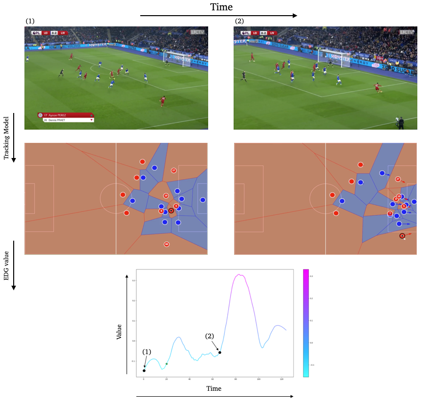
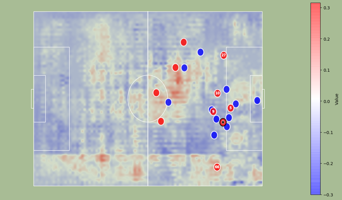
Evolution of our Tracking and EDG model over time. The EDG model learns to capture actions with potential in a very general manner, and compute such potential with the player coordinates our Tracking model gathers from the live Camera.
This blog post is the markdown version of a list of Jupyter Notebooks you can find inside Narya’s repository. This post allows to have each Notebook at the same place. It will probably be replaced by a Jupyter Book whenever I find the time and the solution to integrate them into this blog.
We tried to make everything easy to reuse, we hope anyone will be able to:
Use our datasets to train other models
Finetune some of our trained models
Use our trackers
Evaluate players with our EDG Agent
and much more
I now work at Flaneer, feel free to reach out if you are interested!
Narya
The Narya API allows you to track soccer player from camera inputs, and evaluate them with an Expected Discounted Goal (EDG) Agent. This repository contains the implementation of the following paper. We also make available all of our trained agents, and the datasets we used as well.
This Notebook’s goal is to allow anyone without any access to soccer data to produce its own and analyze them with powerful tools. We also hope that by releasing our training procedures and datasets, better models will emerge and make this tool better iteratively.
Framework
Our library is split in 2: one part is to track soccer players, another one is to process these trackings and evaluate them. Let’s start by focusing on how to track soccer players.
Installation
git clone && cd narya && pip3 install -r requirements.txt
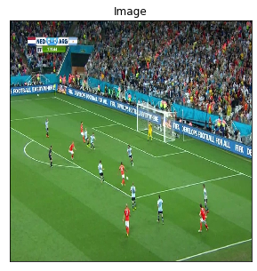
Let’s start by importing some libraries and an image we will use during this Notebook:
(a) The ET model computes the position of each entity. It then passes the coordinates to the online tracker to: (1): Compute the embedding of each player, (2): Warp each coordinate with the homography from HE.
(b) The HE starts by doing a direct estimation of the homography. Available keypoints are then predicted and used to compute another estimation of the homography. Both predictions are used to remove potential outliers.
(c) The REID model computes an embedding for each detected player. It also compares the IoU's of each pair of players and applies a Kalman Filter to each trajectory.
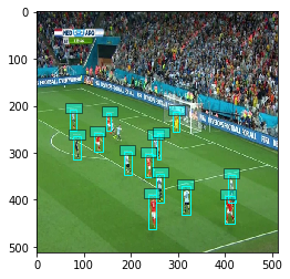
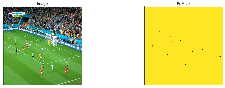
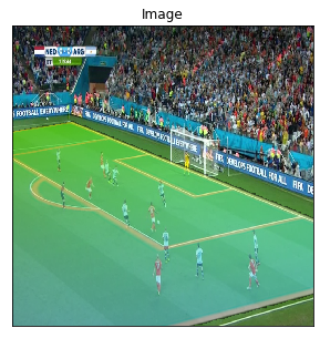
Players detections
The Player Detection model : $\mathbb{R} ^ {n \times n \times 3} \to \mathbb{R} ^ {m \times 4} \times \left[0,1\right] ^ {m} \times \left[0,1\right] ^ {m}$, takes an image as input, and predicts a list of bounding boxes associated with a class prediction (Player or Ball) and a confidence value. The model is based on a Single Shot MultiBox Detector (SSD), with an implementation from GluonCV.
You can easily:
Load the model
Load weights for this model
Call this model
We tried to keep a similar architecture for each model, even with a different framework.
For example, each model deals on itself with image preprocessing, reshaping, and so on: a simple __call__ is enough.
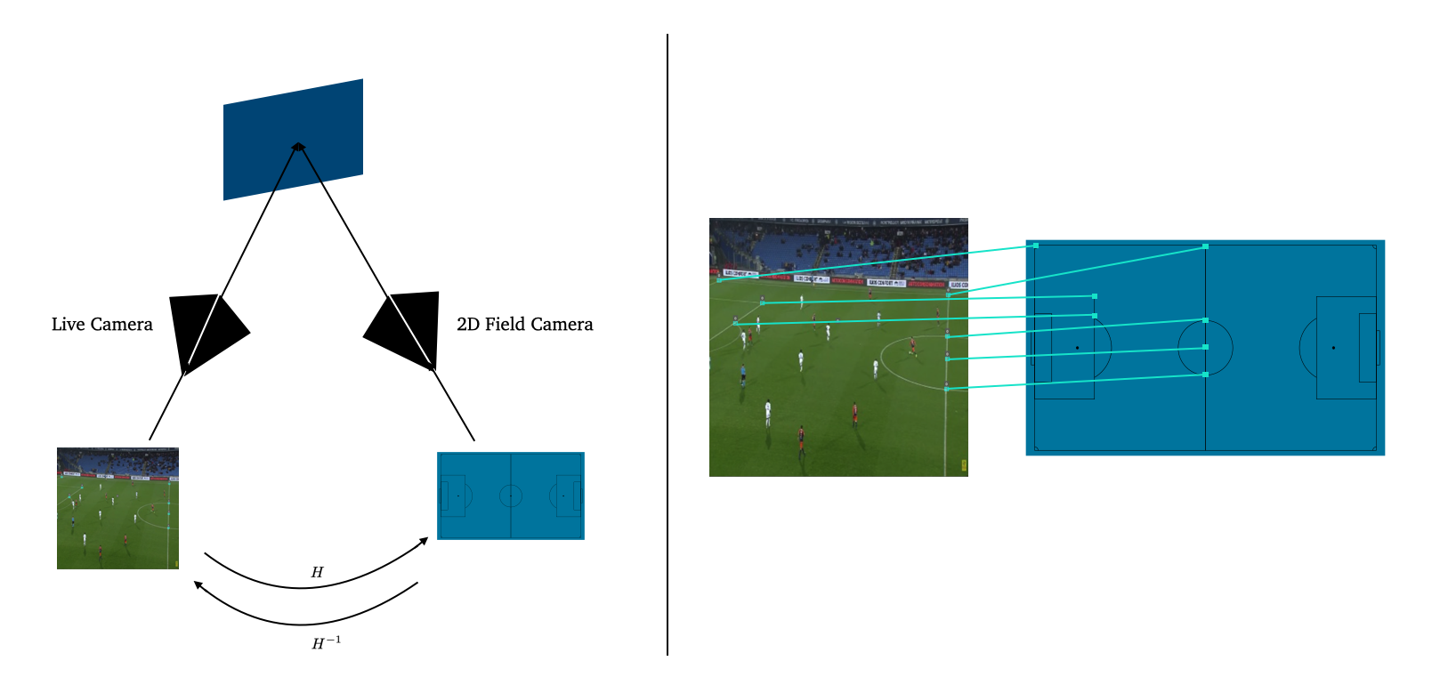
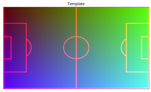
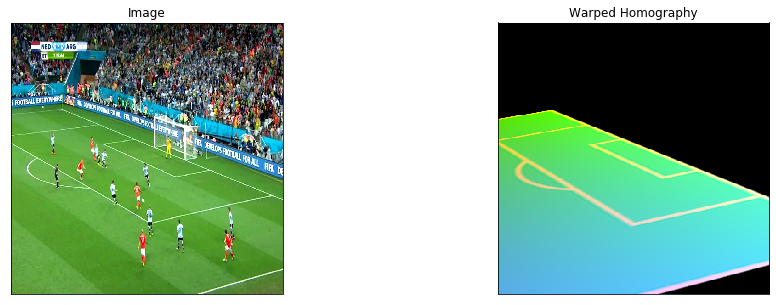
Now that we have players’ coordinates (and the ball position), we need to be able to transform them into 2D coordinates. This means finding the homography between our input image and a 2D representation of the field:
(left) Example of a planar surface (our soccer field) viewed by two camera positions: the 2D field camera and the Live camera. Finding the homography between them allows to produce 2D coordinates for each player.
(right) Example of points correspondences between the 2D Soccer Field Camera and the Live Camera.
Homography Estimations
We developed 2 methods to ensure more robust estimations of the current homography. The first one is a direct prediction, and the second one computes the homography from the detection of some particular keypoints. Let’s start with the direct prediction: $\mathbb{R} ^ {n \times n \times 3} \to \mathbb{R} ^ {3 \times 3}$.
The model is based on a Resnet-18 architecture and takes images of shape $(280,280)$. It was implemented with Keras. Let’s review its architecture, which is kept the same for each model, no matter its framework.
Each model is created with:
The shape of its input
If we want it pretrained or not
It then creates a model and a preprocessing function:
classDeepHomoModel:"""Class for Keras Models to predict the corners displacement from an image. These corners can then get used
to compute the homography.
Arguments:
pretrained: Boolean, if the model is loaded pretrained on ImageNet or not
input_shape: Tuple, shape of the model's input
Call arguments:
input_img: a np.array of shape input_shape
"""def__init__(self,pretrained=False,input_shape=(256,256)):self.input_shape=input_shapeself.pretrained=pretrainedself.resnet_18=_build_resnet18()inputs=tf.keras.layers.Input((self.input_shape[0],self.input_shape[1],3))x=self.resnet_18(inputs)outputs=pyramid_layer(x,2)self.model=tf.keras.models.Model(inputs=[inputs],outputs=outputs,name="DeepHomoPyramidalFull")self.preprocessing=_build_homo_preprocessing(input_shape)
Our second approach is based on keypoints detection: $\mathbb{R} ^ {n \times n \times 3} \to \mathbb{R} ^ {p \times n \times n}$ we predict $p$ masks, each mask representing a particular keypoint on the field. The homography is computed knowing the coordinates of available keypoints on the image, by mapping them to the keypoints coordinates of the 2-dimensional field. The model is based on an EfficientNetb-3 backbone on top of a Feature Pyramid Networks (FPN) architecture to predict each keypoint’s mask. We implemented our model using Segmentation Models.
Again, let’s start by quickly creating our model and making some predictions:
Here, we display a concatenation of each keypoints we predicted. Now, since we know the “true” coordinates of each of them, we can precisely compute the related homography parameters.
Notes: We explain here how the homography parameters are computed. This is a Supplementary Material from our paper and, therefore, can be skipped.
We assume 2 sets of points $(x_1,y_1)$ and $(x_2,y_2)$ both in $\mathbb{R}^2$, and define $\mathbf{X_i}$ as $[x_i,y_i,1]^{\top}$. We define the planar homography $\mathbf{H}$ that relates the transformation between the 2 planes generated by $\mathbf{X_1}$ and $\mathbf{X_2}$ as :
where we assume $h_{33} = 1$ to normalize $\mathbf{H}$ and since $\mathbf{H}$ only has $8$ degrees of freedom as it estimates only up to a scale factor. The equation above yields the following 2 equations:
where $\mathbf{h} = [h_{11},h_{12},h_{13},h_{21},h_{22},h_{23},h_{31},h_{32}]^{\top}$. We can stack such constraints for $n$ pair of points, leading to a system of equations of the form $\mathbf{A}\mathbf{h} = 0$ where $\mathbf{A}$ is a $2n \times 8$ matrix. Given the $8$ degrees of freedom and the system above, we need at least $8$ points (4 in each plan) to compute an estimation of our homography.
This is the method we use to compute the homography from the keypoints prediction.
Let’s do it and predict an homography from these keypoints:
In the next section, we will see how to use all of these models together to track players on a video.
Online Tracking
Given a list of images, we want to track players and the ball and gather their trajectories. Our model initializes several tracklets based on the detected boxes in the first image. In the following ones, the model links the boxes to the existing tracklets according to:
their distance measured by the embedding model,
their distance measured by boxes IoU’s
When the entire list of images is processed, we compute a homography for each image. We then apply each homography to the player’s coordinates.
"""
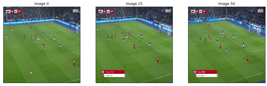
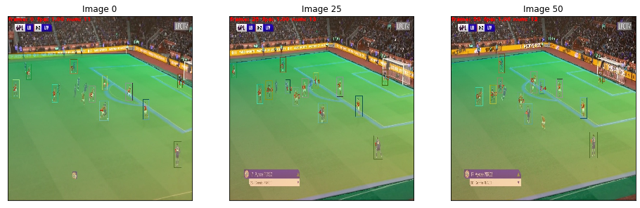
Images are ordered from 0 to 50:
"""imgs_ordered=[]foriinrange(0,51):path='test_img/img_fullLeicester 0 - [3] Liverpool.mp4_frame_full_'+str(i)+'.jpg'imgs_ordered.append(path)img_list=[]forpathinimgs_ordered:ifpath.endswith('.jpg'):image=cv2.imread(path)image=cv2.cvtColor(image,cv2.COLOR_BGR2RGB)img_list.append(image)
We first need to create our tracker. This object gathers every one of our models:
classFootballTracker:"""Class for the full Football Tracker. Given a list of images, it allows to track and id each player as well as the ball.
It also computes the homography at each given frame, and apply it to each player coordinates.
Arguments:
pretrained: Boolean, if the homography and tracking models should be pretrained with our weights or not.
weights_homo: Path to weight for the homography model
weights_keypoints: Path to weight for the keypoints model
shape_in: Shape of the input image
shape_out: Shape of the ouput image
conf_tresh: Confidence treshold to keep tracked bouding boxes
track_buffer: Number of frame to keep in memory for tracking reIdentification
K: Number of boxes to keep at each frames
frame_rate: -
Call arguments:
imgs: List of np.array (images) to track
split_size: if None, apply the tracking model to the full image. If its an int, the image shape must be divisible by this int.
We then split the image to create n smaller images of shape (split_size,split_size), and apply the model
to those.
We then reconstruct the full images and the full predictions.
results: list of previous results, to resume tracking
begin_frame: int, starting frame, if you want to resume tracking
verbose: Boolean, to display tracking at each frame or not
save_tracking_folder: Foler to save the tracking images
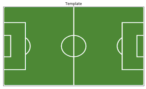
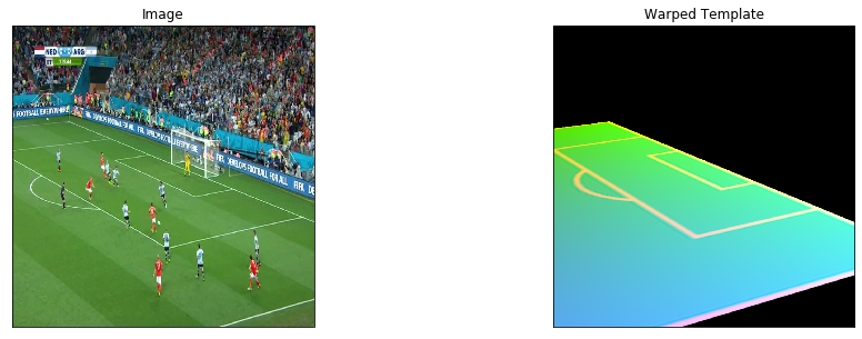
template: Football field, to warp it with the computed homographies on to the saved images
skip_homo: List of int. e.g.: [4,10] will not compute homography for frame 4 and 10, and reuse the computed homography
at frame 3 and 9.
"""def__init__(self,pretrained=True,weights_homo=None,weights_keypoints=None,shape_in=512.0,shape_out=320.0,conf_tresh=0.5,track_buffer=30,K=100,frame_rate=30,):self.player_ball_tracker=PlayerBallTracker(conf_tresh=conf_tresh,track_buffer=track_buffer,K=K,frame_rate=frame_rate)self.homo_estimator=HomographyEstimator(pretrained=pretrained,weights_homo=weights_homo,weights_keypoints=weights_keypoints,shape_in=shape_in,shape_out=shape_out,)
Creating model...
Succesfully loaded weights from /Users/paulgarnier/.keras/datasets/player_tracker.params
Succesfully loaded weights from /Users/paulgarnier/.keras/datasets/player_reid.pth
WARNING:tensorflow:No training configuration found in the save file, so the model was *not* compiled. Compile it manually.
Succesfully loaded weights from /Users/paulgarnier/.keras/datasets/deep_homo_model.h5
Succesfully loaded weights from /Users/paulgarnier/.keras/datasets/keypoint_detector.h5
We now only have to call it on our list of images. We manually remove some failed homography estimation, at frame $\in {25,…,30 }$ by adding skip_homo = [25,26,27,28,29,30] into our call.
100% (51 of 51) |########################| Elapsed Time: 0:00:00 Time: 0:00:00
Process trajectories
We now have raw trajectories that we need to process.
Fist, you can do several operations to ensure that the trajectories are functional:
Delete an id at a specific frame
Delete an id from every frame
Merge two ids
Add an id at a given frame
These operations are simple to do with some of our functions from narya.utils.tracker:
def_remove_coords(traj,ids,frame):"""Remove the x,y coordinates of an id at a given frame
Arguments:
traj: Dict mapping each id to a list of trajectory
ids: the id to target
frame: int, the frame we want to remove
Returns:
traj: Dict mapping each id to a list of trajectory
Raises:
"""def_remove_ids(traj,list_ids):"""Remove ids from a trajectory
Arguments:
traj: Dict mapping each id to a list of trajectory
list_ids: List of id
Returns:
traj: Dict mapping each id to a list of trajectory
Raises:
"""defadd_entity(traj,entity_id,entity_traj):"""Adds a new id with a trajectory
Arguments:
traj: Dict mapping each id to a list of trajectory
entity_id: the id to add
entity_traj: the trajectory linked to entity_id we want to add
Returns:
traj: Dict mapping each id to a list of trajectory
Raises:
"""defadd_entity_coords(traj,entity_id,entity_traj,max_frame):"""Add some coordinates to the trajectory of a given id
Arguments:
traj: Dict mapping each id to a list of trajectory
entity_id: the id to target
entity_traj: List of (x,y,frame) to add to the trajectory of entity_id
max_frame: int, the maximum number of frame in trajectories
Returns:
traj: Dict mapping each id to a list of trajectory
Raises:
"""defmerge_id(traj,list_ids_frame):"""Merge trajectories of different ids.
e.g.: (10,0,110),(12,110,300) will merge the trajectory of 10 between frame 0 and 110 to the
trajectory of 12 between frame 110 and 300.
Arguments:
traj: Dict mapping each id to a list of trajectory
list_ids_frame: List of (id,frame_start,frame_end)
Returns:
traj: Dict mapping each id to a list of trajectory
Raises:
"""defmerge_2_trajectories(traj1,traj2,id_mapper,max_frame_traj1):"""Merge 2 dict of trajectories, if you want to merge the results of 2 tracking
Arguments:
traj1: Dict mapping each id to a list of trajectory
traj2: Dict mapping each id to a list of trajectory
id_mapper: A dict mapping each id in traj1 to id in traj2
max_frame_traj1: Maximum number of frame in the first trajectory
Returns:
traj1: Dict mapping each id to a list of trajectory
Raises:
"""
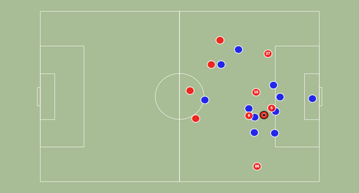
Here, let’s assume we don’t have to perform any operations, and directly process our trajectories into a Pandas Dataframe.
We now have access to a dataframe with for each id, for each frame, the 2D coordinates of the entity.
df.head()
id
x
y
frame
1
1
78.251729
10.133520
2
1
78.262442
10.138342
3
1
78.308051
10.483425
4
1
78.356691
10.792084
5
1
78.379051
10.967897
Finally, this you can save this dataframe using df.to_csv('results_df.csv')
EDG
Now that we have some tracking data, it is time to evaluate them.
Theoretical framework
We assume $s_t \in \mathcal{S}$ is the state of the game at time $t$. It may be the positions of each player and the ball for example. Given an action $a \in \mathcal{A}$ (\eg a pass, a shot,etc), and a state $s’ \in \mathcal{S}$, we note $\mathbb{P} \colon \mathcal{S} \times \mathcal{A} \times \mathcal{S} \to [0,1]$ the probability $\mathbb{P} (s’ \vert s, a)$ of getting to state $s’$ from $s$ following action $a$.
%
Applying actions over $K$ time steps yields a trajectory of states and actions, $\tau ^{t_{0:K}} = \big(s_{t_0},a_{t_0}, … ,s_{t_K},a_{t_K} \big)$. We denote $r_t$ the reward given going from $s_t$ to $s_{t+1}$ (\eg $+1$ if the team scores a goal). More importantly, the cumulative discounted reward along $\tau ^{t_{0:K}}$ is defined as:
where $\gamma \in \left[0,1\right]$ is a discount factor, smoothing the impact of temporally distant rewards.
A policy, $\pi _{\theta}$, chooses the action at any given state, whose parameters, $\theta$, can be optimized for some training objectives (such as maximizing $R$). Here, a good policy would be a policy representing the team we want to analyze in the right manner. The \textit{Expected Discounted Goal} (EDG), or more generally, the state value function, is defined as:
\[V^\pi (s) = \underset{\tau \sim \pi}{\mathbb{E}} \big[ R(\tau) \vert s \big]\]
It represents the discounted expected number of goals the team will score (or concede) from a particular state. To build such a good policy, one can define an objective function based on the cumulative discounted reward:
To that end, we can compute the gradient of such cost function\footnote{Using a log probability trick, we can show that we have the following equality: $\nabla_\theta J(\theta) = \underset{\tau \sim \pi_\theta}{\mathbb{E}} \left[ \sum_{t=0}^T \nabla_\theta \log \left( \pi_\theta (a_t \vert s_t) \right) R(\tau) \right]$} $\nabla_\theta J(\theta)$ to update our parameters with $\theta \leftarrow \theta + \lambda \nabla_\theta J(\theta)$. In our case, the evaluation of $V^\pi$ and $\pi_\theta$ is done using Neural Networks, and $\theta$ represents the weights of such networks. At inference, our model will take the state of the game as input, and will output the estimation of the EDG.
Implementation
Our EDG agent was implemented using the Google Football library. We trained our agent against bots and against itself until it became strong enough. Such an agent can be seen on this youtube video.
Let’s start by importing some libraries:
Notes: Google Football is not compatible with Tensorflow 2 yet. We have to downgrade it to use our agent.
Homography Dataset: The homography dataset is made of pair of images,matrix in a .jpg,.npy format. The matrix is the homography associated with the image. They are normalized, meaning that homography[2,2] == 1.
Keypoints Dataset: We give here pair of images,xml file. The .xml files are made of the coordinates of each available keypoints on the image. We built utils function to read these files, and do so automaticaly in our Dataset class.
Tracking Dataset: Pair of images,xml files in a VOC format.
Training
Finally, we give here a quick tour of our training scripts.
# define optomizer
optim=keras.optimizers.Adam(opt.lr)# define loss function
dice_loss=sm.losses.DiceLoss()focal_loss=sm.losses.CategoricalFocalLoss()total_loss=dice_loss+(1*focal_loss)metrics=[sm.metrics.IOUScore(threshold=0.5),sm.metrics.FScore(threshold=0.5)]# compile keras model with defined optimozer, loss and metrics
model.compile(optim,total_loss,metrics)callbacks=[keras.callbacks.ModelCheckpoint(name_model,save_weights_only=True,save_best_only=True,mode="min"),keras.callbacks.ReduceLROnPlateau(patience=10,verbose=1,cooldown=10,min_lr=0.00000001),]model.summary()
We can easily build a Dataset and a Dataloader (handling batches):

 Number of invocation of the “join another session” function