Football Data Analysis - Liverpool FC attacking system

This post was made possible by @lastrowview and @Soccermatics which shared the tracking data of 19 goals scored by LFC during 2018–2019 and 2019-2020 seasons. Our code is available on this GitHub repository.

This article was co-written with Théophane, a classmate, while we worked on this project for a few days.

I now work at Flaneer, feel free to reach out if you are interested!

This post illustrates how data analysis and machine learning can be applied to football players’ tracking data in order to reveal key insights. Our analysis will be articulated in two parts :

• Pitch control for opponent analysis
• Deep Reinforcement Learning (DRL) for accessing action value

Pitch control for opponent analysis

A pitch control model basically tells you which team is in control of every pitch part at a given time. Here, “in control” means being the quicker to arrive at a specific location in case the ball is shot there.

Starting from position data, we got access to speed data thanks to discrete derivation and Savitzky–Golay filter. Then, our approach was to use a time-based Voronoi tessellation operating with ball and players’ tracking data (positions and speeds) as inputs and physical characteristics (player maximum speed, reaction time…) as parameters. This model is an adaptation from the one developed by Laurie Shaw (Harvard) for Metrica’s tracking data.

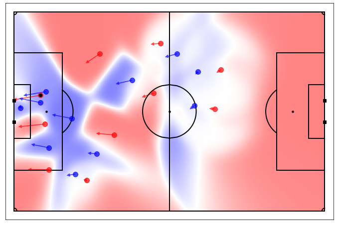
After calculating pitch control map frame per frame, we were then able to produce video analysis like this one :

Wing-backs : the two lungs of Liverpool’s attack

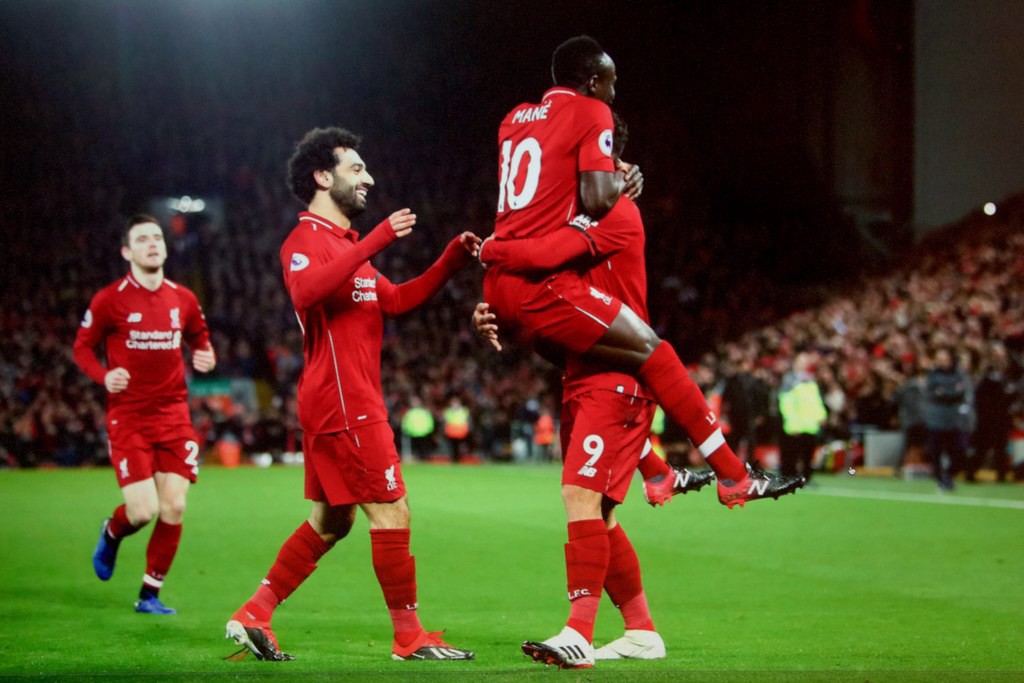
Football analysts often emphasize on LFC amazing attacking trio : Mané, Salah and Firmino. In fact, the two wing-backs, Andrew Robertson and Trent Alexander-Arnold, play an offensive role almost as significant as the famous trio.

Analyzing the Reds goals, their attacking system seems to focus on the wings in order to get around the defensive line. Indeed, most of the goals are coming from either curved passes (and crosses) or diving runs from outside to inside.

Our pitch control model enabled us to illustrate space creation by wing-backs such as this triggering run from Alexander-Arnold against Porto FC.

This attacking system is based on speed and quick decisions as opposed to more centered playing styles creating a nexus of short passes such as Guardiola’s FC Bayern Munich from 2015–2016 season (or even more in 2010 during Barcelona FC golden age). Therefore, defenders’ response time must be extremely short to counteract the Reds and reach a clean sheet.

Defenders’ response time : every second is precious against LFC

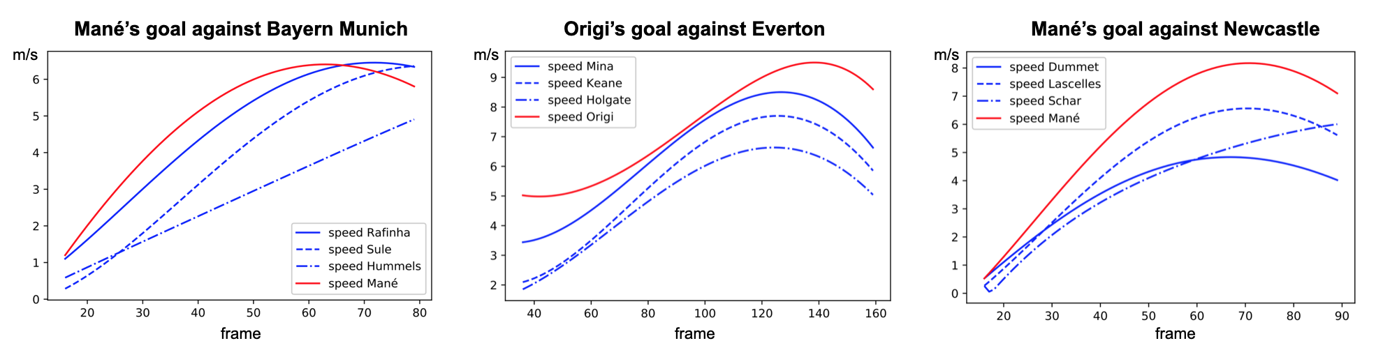
At first sight, these graphs just seem to show that attacking players are faster than defending players which is not surprising. However, the important point we would like to highlight is the time taken by defenders to reach the attacker’s initial speed. Defenders from Bayern and Everton seem to take a lot more time to react whereas the ones from Newcastle were very reactive (but victim of a huge space between their two center-backs).

The three goals are available here as the support of this analysis.

This pitch control model enables to produce some insights on the game. Now, let’s see how we can value actions thanks to Deep Reinforcement Learning.

Deep Reinforcement Learning Agent

An important aspect of football analysis is the concept of expected goals (xG). An overview can be found here, with several references as well. We adapt this concept here to the Reinforcement Learning framework, considering a football game as a Markov Decision Process. At its core, reinforcement learning models an agent interacting with an environment and receiving observations and rewards from it. The goal of an agent is to determine the best action in any given state. In the case of football, we could consider :

• An episode as one game.
• A state as the position and velocity of each player and the ball.
• Possible actions as a player moving or making a pass.
• The reward as +1 if we score a goal, -1 if we conceded one.

One adaptation of the Reinforcement Learning framework to football can be found here.

A few mathematics considerations

We define a trajectory $\tau$ as a sequence of states and actions experienced by the agent :

and we define the discounted cumulative reward as the gain along a trajectory :

where $\gamma$ is a discount factor, and $r_t$ the reward at time $t$. 

Finally, we define the state value function according to a policy $\pi$ (the way the agent behave) as : 

This value function can represent the expected discounted cumulative reward starting from a state $s$ and following a given policy $\pi$. Since, in our framework, we only get a reward when the agent scores a goal, we can interpret $V(s)$ as the expected discounted goals from a given state.

Granted, you would need a policy or an agent that can play the same way the players you are targetting, and that is a complicated issue to tackle. We used here the Google Research Football environment to train our agents and used their hyper-parameters (except for the reward, we used the scoring reward):

--level 11_vs_11_easy_stochastic \
  --reward_experiment scoring \
  --policy impala_cnn \
  --cliprange 0.08 \
  --gamma 0.993 \
  --ent_coef 0.003 \
  --num_timesteps 50000000 \
  --max_grad_norm 0.64 \
  --lr 0.000343 \
  --num_envs 16 \
  --noptepochs 2 \
  --nminibatches 8 \
  --nsteps 512 \

We also kept training our agent against middle and hard opponents overtime and finished the training with self-play. We release the checkpoint used for the value function evaluation in our repository.

Finally, we wanted to fine-tune our agent with some Imitation Learning, by using real games data. However, due to the lack of time, this did not happen. It will be the next step for this particular project. We will also need to conduct a more thorough analysis of the differences between this approach and the more usual Expected Goals models. A multi-agent approach might also bring some value to this application, with a more precise prediction of the Expected Discounted Goals.

Results

We convert the tracking data from Last Row into a readable format for our agent :

“The observation is composed of 4 planes of size ‘channel_dimensions’. Its size is then ‘channel_dimensions’x4 (or ‘channel_dimensions’x16 when stacked is True). The first plane P holds the position of players on the left team, P(y,x) is 255 if there is a player at position (x,y), otherwise, its value is 0. The second plane holds in the same way the position of players on the right team. The third plane holds the position of the ball. The last plane holds the active player.” extracted from Google Research Football GitHub

that are stacked for four frames.

We then compute the value function for each time step and smooth it using a Savitzky-Golay filter. We apply our value function to a goal against Leicester. The results are available below :

Without over-analyzing the value function, a few things are still interesting to notice :

• The pass between time frames 20–30 increases a lot the value function, as well as the assist from Alexander-Arnold.
• Overall, the entire action on the right side brings a lot of value.
• The value function decreases before the shot (as the agent believes that the action is compromised) and after the goal (since such a configuration is never seen within the simulation)

Conclusion

Through this post, we tried to find interesting approaches to Liverpool FC tracking data and we are fully aware our analysis is not complete. We still had a lot of fun working on the dataset provided by @lastrowview and we would also like to thank Friends of Tracking youtube channel for sharing useful repositories and gathering knowledge on Football Data Analysis.