Narya - Tracking and Evaluating Soccer Players
This blog post is the markdown version of a list of Jupyter Notebooks you can find inside Narya’s repository. This post allows to have each Notebook at the same place. It will probably be replaced by a Jupyter Book whenever I find the time and the solution to integrate them into this blog.
This project is also an evolution from a previous blog post.
We tried to make everything easy to reuse, we hope anyone will be able to:
- Use our datasets to train other models
- Finetune some of our trained models
- Use our trackers
- Evaluate players with our EDG Agent
- and much more
I now work at Flaneer, feel free to reach out if you are interested!
Narya
The Narya API allows you to track soccer player from camera inputs, and evaluate them with an Expected Discounted Goal (EDG) Agent. This repository contains the implementation of the following paper. We also make available all of our trained agents, and the datasets we used as well.
This Notebook’s goal is to allow anyone without any access to soccer data to produce its own and analyze them with powerful tools. We also hope that by releasing our training procedures and datasets, better models will emerge and make this tool better iteratively.
Framework
Our library is split in 2: one part is to track soccer players, another one is to process these trackings and evaluate them. Let’s start by focusing on how to track soccer players.
Installation
git clone && cd narya && pip3 install -r requirements.txt
Let’s start by importing some libraries and an image we will use during this Notebook:
!pip3 install --user tensorflow==2.2.0
!pip3 install --upgrade --user tensorflow-probability
!pip3 install --upgrade --user dm-sonnet
import numpy as np
import cv2
from matplotlib import pyplot as plt

from narya.utils.vizualization import visualize
image = cv2.imread('test_image.jpg')
image = cv2.cvtColor(image, cv2.COLOR_BGR2RGB)
print("Image shape: {}".format(image.shape))
visualize(image=image)
Tracking Soccer Players
![]()
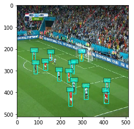
Players detections
The Player Detection model : $\mathbb{R} ^ {n \times n \times 3} \to \mathbb{R} ^ {m \times 4} \times \left[0,1\right] ^ {m} \times \left[0,1\right] ^ {m}$, takes an image as input, and predicts a list of bounding boxes associated with a class prediction (Player or Ball) and a confidence value. The model is based on a Single Shot MultiBox Detector (SSD), with an implementation from GluonCV.
You can easily:
- Load the model
- Load weights for this model
- Call this model
We tried to keep a similar architecture for each model, even with a different framework.
For example, each model deals on itself with image preprocessing, reshaping, and so on: a simple __call__ is enough.
Let’s start by importing a tracking model:
from narya.models.gluon_models import TrackerModel
from gluoncv.utils import viz
import tensorflow as tf

tracker_model = TrackerModel(pretrained=True, backbone='ssd_512_resnet50_v1_coco')
and load our pre-trained weights:
Note: When a TrackerModel gets instantiate more than once, weights won’t load successfully. Make sure to restart the kernel in this case.
WEIGHTS_PATH = (
    "https://storage.googleapis.com/narya-bucket-1/models/player_tracker.params"
)
WEIGHTS_NAME = "player_tracker.params"
WEIGHTS_TOTAR = False

checkpoints = tf.keras.utils.get_file(
                WEIGHTS_NAME, WEIGHTS_PATH, WEIGHTS_TOTAR,
            )

tracker_model.load_weights(checkpoints)
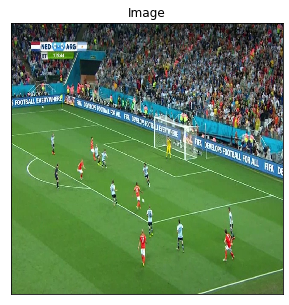
You can now easily use this model to make predictions on any soccer related images. Let’s try it on our example:
cid, score, bbox = tracker_model(image, split_size = 512)
ax = viz.plot_bbox(cv2.resize(image,(512,512)), bbox[0], score[0], cid[0], class_names=tracker_model.model.classes,thresh=0.5,linewidth=1,fontsize=1)
plt.show()
Now that we have players’ coordinates (and the ball position), we need to be able to transform them into 2D coordinates. This means finding the homography between our input image and a 2D representation of the field:
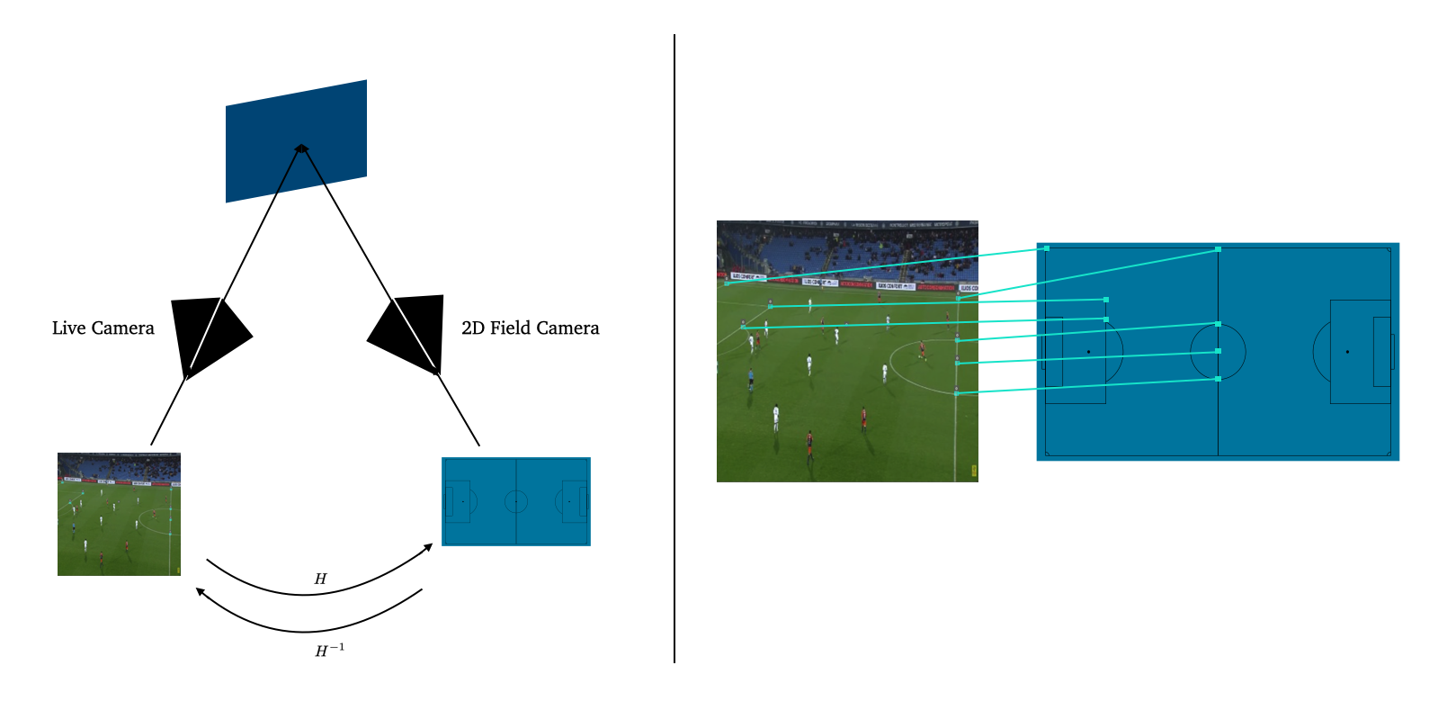
Homography Estimations
We developed 2 methods to ensure more robust estimations of the current homography. The first one is a direct prediction, and the second one computes the homography from the detection of some particular keypoints. Let’s start with the direct prediction: $\mathbb{R} ^ {n \times n \times 3} \to \mathbb{R} ^ {3 \times 3}$.
The model is based on a Resnet-18 architecture and takes images of shape $(280,280)$. It was implemented with Keras. Let’s review its architecture, which is kept the same for each model, no matter its framework.
Each model is created with:
- The shape of its input
- If we want it pretrained or not
It then creates a model and a preprocessing function:
class DeepHomoModel:
    """Class for Keras Models to predict the corners displacement from an image. These corners can then get used
    to compute the homography.

    Arguments:
        pretrained: Boolean, if the model is loaded pretrained on ImageNet or not
        input_shape: Tuple, shape of the model's input
    Call arguments:
        input_img: a np.array of shape input_shape
    """

    def __init__(self, pretrained=False, input_shape=(256, 256)):

        self.input_shape = input_shape
        self.pretrained = pretrained

        self.resnet_18 = _build_resnet18()

        inputs = tf.keras.layers.Input((self.input_shape[0], self.input_shape[1], 3))
        x = self.resnet_18(inputs)
        outputs = pyramid_layer(x, 2)

        self.model = tf.keras.models.Model(
            inputs=[inputs], outputs=outputs, name="DeepHomoPyramidalFull"
        )

        self.preprocessing = _build_homo_preprocessing(input_shape)
Each model then has the same call function:
def __call__(self, input_img):

    img = self.preprocessing(input_img)
    corners = self.model.predict(np.array([img]))

    return corners
Let’s apply this direct homography estimation to our example. This can be done easily, exactly like the tracking model:
from narya.models.keras_models import DeepHomoModel

deep_homo_model = DeepHomoModel()

WEIGHTS_PATH = (
    "https://storage.googleapis.com/narya-bucket-1/models/deep_homo_model.h5"
)
WEIGHTS_NAME = "deep_homo_model.h5"
WEIGHTS_TOTAR = False

checkpoints = tf.keras.utils.get_file(
                WEIGHTS_NAME, WEIGHTS_PATH, WEIGHTS_TOTAR,
            )

deep_homo_model.load_weights(checkpoints)

corners = deep_homo_model(image)
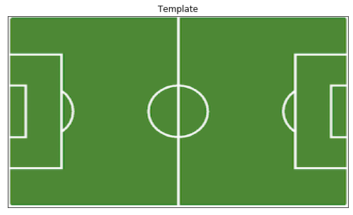
Let’s load a “template” image, a 2D view of the field. This is the image to which we will apply our predicted homography:
template = cv2.imread('world_cup_template.png')
template = cv2.cvtColor(template, cv2.COLOR_BGR2RGB)
template = cv2.resize(template, (1280,720))/255.
visualize(template=template)
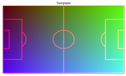
and let’s make it easier to display on another image:
from narya.utils.vizualization import rgb_template_to_coord_conv_template

template = rgb_template_to_coord_conv_template(template)
visualize(template=template)
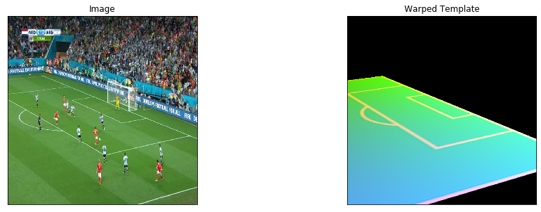
Now, let’s import some utils functions, and warp our template with our predicted homography:
from narya.utils.homography import compute_homography, warp_image,warp_point
from narya.utils.image import torch_img_to_np_img, np_img_to_torch_img, denormalize
from narya.utils.utils import to_torch

pred_homo = compute_homography(corners)[0]
pred_warp = warp_image(np_img_to_torch_img(template),to_torch(pred_homo),method='torch')
pred_warp = torch_img_to_np_img(pred_warp[0])
visualize(image=image,warped_template=cv2.resize(pred_warp, (1024,1024)))
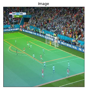
You can also merge the warped template with your example:
Notes: Usually, this homography is only used to compute the coordinates of each player.
from narya.utils.vizualization import merge_template

test = merge_template(image/255.,cv2.resize(pred_warp, (1024,1024)))
visualize(image = test)
Our second approach is based on keypoints detection: $\mathbb{R} ^ {n \times n \times 3} \to \mathbb{R} ^ {p \times n \times n}$ we predict $p$ masks, each mask representing a particular keypoint on the field. The homography is computed knowing the coordinates of available keypoints on the image, by mapping them to the keypoints coordinates of the 2-dimensional field. The model is based on an EfficientNetb-3 backbone on top of a Feature Pyramid Networks (FPN) architecture to predict each keypoint’s mask. We implemented our model using Segmentation Models.
Again, let’s start by quickly creating our model and making some predictions:
from narya.models.keras_models import KeypointDetectorModel

kp_model = KeypointDetectorModel(
    backbone='efficientnetb3', num_classes=29, input_shape=(320, 320),
)

WEIGHTS_PATH = (
    "https://storage.googleapis.com/narya-bucket-1/models/keypoint_detector.h5"
)
WEIGHTS_NAME = "keypoint_detector.h5"
WEIGHTS_TOTAR = False

checkpoints = tf.keras.utils.get_file(
                WEIGHTS_NAME, WEIGHTS_PATH, WEIGHTS_TOTAR,
            )

kp_model.load_weights(checkpoints)

pr_mask = kp_model(image)
visualize(
        image=denormalize(image.squeeze()),
        pr_mask=pr_mask[..., -1].squeeze(),
    )
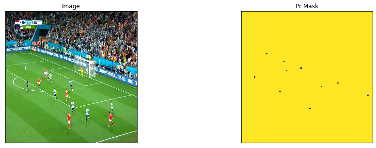
Here, we display a concatenation of each keypoints we predicted. Now, since we know the “true” coordinates of each of them, we can precisely compute the related homography parameters.
Notes: We explain here how the homography parameters are computed. This is a Supplementary Material from our paper and, therefore, can be skipped.
We assume 2 sets of points $(x_1,y_1)$ and $(x_2,y_2)$ both in $\mathbb{R}^2$, and define $\mathbf{X_i}$ as $[x_i,y_i,1]^{\top}$. We define the planar homography $\mathbf{H}$ that relates the transformation between the 2 planes generated by $\mathbf{X_1}$ and $\mathbf{X_2}$ as :
\[\mathbf{X_2} = \mathbf{H}\mathbf{X_1} = \begin{bmatrix} h_{11} & h_{12} & h_{13} \\ h_{21} & h_{22} & h_{23} \\ h_{31} & h_{32} & h_{33} \end{bmatrix} \mathbf{X_1}\]where we assume $h_{33} = 1$ to normalize $\mathbf{H}$ and since $\mathbf{H}$ only has $8$ degrees of freedom as it estimates only up to a scale factor. The equation above yields the following 2 equations:
\[x_2 = \frac{h_{11}x_1 + h_{12}y_1 + h_{13}}{h_{31}x_1 + h_{32}y_1 + 1}\] \[y_2 = \frac{h_{21}x_1 + h_{22}y_1 + h_{23}}{h_{31}x_1 + h_{32}y_1 + 1}\]that we can rewrite as :
\[x_2 = h_{11}x_1 + h_{12}y_1 + h_{13} - h_{31}x_1x_2 - h_{32}y_1x_2\] \[y_2 = h_{21}x_1 + h_{22}y_1 + h_{23} - h_{31}x_1y_2 - h_{32}y_1y_2\]or more concisely:
\[\begin{bmatrix} x_1 & y_1 & 1 & 0 & 0 & 0 & -x_1x_2 & -y_1x_2 \\ 0 & 0 & 0 & x_1 & y_1 & 1 & -x_1y_2 & -y_1y_2 \end{bmatrix} \mathbf{h} = 0\]where $\mathbf{h} = [h_{11},h_{12},h_{13},h_{21},h_{22},h_{23},h_{31},h_{32}]^{\top}$. We can stack such constraints for $n$ pair of points, leading to a system of equations of the form $\mathbf{A}\mathbf{h} = 0$ where $\mathbf{A}$ is a $2n \times 8$ matrix. Given the $8$ degrees of freedom and the system above, we need at least $8$ points (4 in each plan) to compute an estimation of our homography.
This is the method we use to compute the homography from the keypoints prediction.
Let’s do it and predict an homography from these keypoints:
from narya.utils.masks import _points_from_mask
from narya.utils.homography import get_perspective_transform
src,dst = _points_from_mask(pr_mask[0])
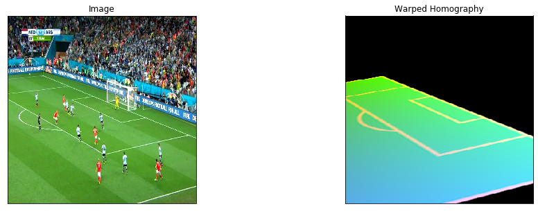
pred_homo = get_perspective_transform(dst,src)
pred_warp = warp_image(cv2.resize(template, (320,320)),pred_homo,out_shape=(320,320))
visualize(
image=denormalize(image.squeeze()),
warped_homography=pred_warp,
)
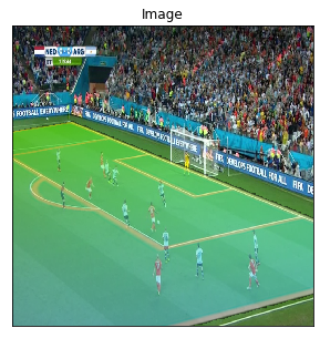
and if we merge them:
test = merge_template(image/255.,cv2.resize(pred_warp, (1024,1024)))
visualize(image = test)
ReIdentification
Finally, we need to be able to say if one player from the first frame is the same in another frame. We use three tools to do so:
- a Kalman filter, to remove outliers
- the IoU distance, to ensure that one person cannot move too much in 2 consecutive frames
- the cosine similarity between embeddings
Our last model deals with the embedding part. Once again, even as a torch model, it can be loaded and used as the rest.
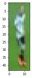
Let’s start by cropping the image of a player:
x_1 = int(bbox[0][0][0])
y_1 = int(bbox[0][0][1])
x_2 = int(bbox[0][0][2])
y_2 = int(bbox[0][0][3])
print(x_1,x_2,y_1,y_2)

resized_image = cv2.resize(image,(512,512))
plt.imshow(resized_image[y_1:y_2,x_1:x_2])
Now, we can create and call our model:
from narya.models.torch_models import ReIdModel

reid_model = ReIdModel()

WEIGHTS_PATH = (
    "https://storage.googleapis.com/narya-bucket-1/models/player_reid.pth"
)
WEIGHTS_NAME = "player_reid.pth"
WEIGHTS_TOTAR = False

checkpoints = tf.keras.utils.get_file(
                WEIGHTS_NAME, WEIGHTS_PATH, WEIGHTS_TOTAR,
            )

reid_model.load_weights(checkpoints)

player_img = resized_image[y_1:y_2,x_1:x_2]
embedding = reid_model(player_img)
In the next section, we will see how to use all of these models together to track players on a video.
Online Tracking
Given a list of images, we want to track players and the ball and gather their trajectories. Our model initializes several tracklets based on the detected boxes in the first image. In the following ones, the model links the boxes to the existing tracklets according to:
- their distance measured by the embedding model,
- their distance measured by boxes IoU’s
When the entire list of images is processed, we compute a homography for each image. We then apply each homography to the player’s coordinates.
Inputs
Let’s start by gathering a list of images:
import mxnet as mx
import os
import numpy as np
import torch
import torch.nn.functional as F

import cv2
from matplotlib import pyplot as plt
from narya.utils.vizualization import visualize

from narya.tracker.full_tracker import FootballTracker
First, we initialize a 2d Field template:
template = cv2.imread('world_cup_template.png')
template = cv2.cvtColor(template, cv2.COLOR_BGR2RGB)
template = cv2.resize(template, (1280,720))
template = template/255.
and then we create our list of images:
"""
Images are ordered from 0 to 50:
"""

imgs_ordered = []
for i in range(0,51):
    path = 'test_img/img_fullLeicester 0 - [3] Liverpool.mp4_frame_full_' + str(i) + '.jpg'
    imgs_ordered.append(path)

img_list = []
for path in imgs_ordered:
    if path.endswith('.jpg'):
        image = cv2.imread(path)
        image = cv2.cvtColor(image, cv2.COLOR_BGR2RGB)
        img_list.append(image)
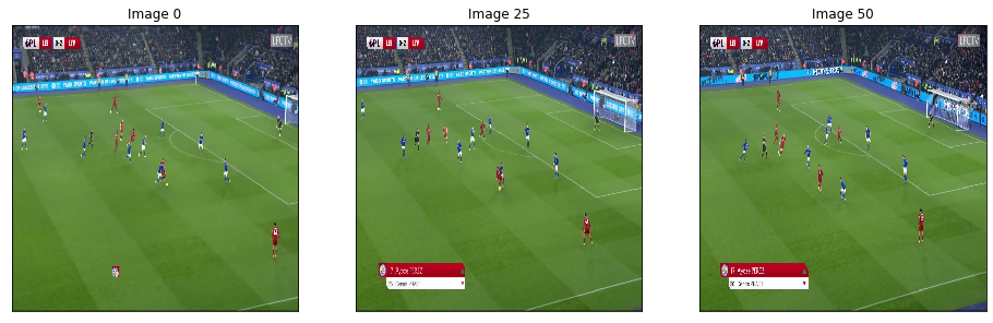
We can vizualize the first image of our list:
image_0,image_25,image_50 = img_list[0],img_list[25],img_list[50]
print("Image shape: {}".format(image_0.shape))
visualize(image_0=image_0,
            image_25=image_25,
            image_50=image_50)
Football Tracker
We first need to create our tracker. This object gathers every one of our models:
class FootballTracker:
"""Class for the full Football Tracker. Given a list of images, it allows to track and id each player as well as the ball.
It also computes the homography at each given frame, and apply it to each player coordinates.

Arguments:
    pretrained: Boolean, if the homography and tracking models should be pretrained with our weights or not.
    weights_homo: Path to weight for the homography model
    weights_keypoints: Path to weight for the keypoints model
    shape_in: Shape of the input image
    shape_out: Shape of the ouput image
    conf_tresh: Confidence treshold to keep tracked bouding boxes
    track_buffer: Number of frame to keep in memory for tracking reIdentification
    K: Number of boxes to keep at each frames
    frame_rate: -
Call arguments:
    imgs: List of np.array (images) to track
    split_size: if None, apply the tracking model to the full image. If its an int, the image shape must be divisible by this int.
                We then split the image to create n smaller images of shape (split_size,split_size), and apply the model
                to those.
                We then reconstruct the full images and the full predictions.
    results: list of previous results, to resume tracking
    begin_frame: int, starting frame, if you want to resume tracking
    verbose: Boolean, to display tracking at each frame or not
    save_tracking_folder: Foler to save the tracking images
    template: Football field, to warp it with the computed homographies on to the saved images
    skip_homo: List of int. e.g.: [4,10] will not compute homography for frame 4 and 10, and reuse the computed homography
                at frame 3 and 9.
"""

    def __init__(
        self,
        pretrained=True,
        weights_homo=None,
        weights_keypoints=None,
        shape_in=512.0,
        shape_out=320.0,
        conf_tresh=0.5,
        track_buffer=30,
        K=100,
        frame_rate=30,
    ):

        self.player_ball_tracker = PlayerBallTracker(
            conf_tresh=conf_tresh, track_buffer=track_buffer, K=K, frame_rate=frame_rate
        )

        self.homo_estimator = HomographyEstimator(
            pretrained=pretrained,
            weights_homo=weights_homo,
            weights_keypoints=weights_keypoints,
            shape_in=shape_in,
            shape_out=shape_out,
        )
tracker = FootballTracker(frame_rate=24.7,track_buffer = 60)
Creating model...
Succesfully loaded weights from /Users/paulgarnier/.keras/datasets/player_tracker.params
Succesfully loaded weights from /Users/paulgarnier/.keras/datasets/player_reid.pth
WARNING:tensorflow:No training configuration found in the save file, so the model was *not* compiled. Compile it manually.
Succesfully loaded weights from /Users/paulgarnier/.keras/datasets/deep_homo_model.h5
Succesfully loaded weights from /Users/paulgarnier/.keras/datasets/keypoint_detector.h5
We now only have to call it on our list of images. We manually remove some failed homography estimation, at frame $\in {25,…,30 }$ by adding skip_homo = [25,26,27,28,29,30] into our call.
trajectories = tracker(img_list,split_size = 512, save_tracking_folder = 'test_outputs/',
                        template = template,skip_homo = [25,26,27,28,29,30])
| |                   #                              | 50 Elapsed Time: 0:00:28


===========Frame 1==========
Activated: [1, 2, 3, 4, 5, 6, 7, 8, 9, 10, 11]
Refind: []
Lost: []
Removed: []

100% (51 of 51) |########################| Elapsed Time: 0:00:00 Time:  0:00:00


===========Frame 51==========
Activated: [1, 3, 9, 20, 4, 7, 13, 24, 5, 10, 8]
Refind: [17]
Lost: []
Removed: []
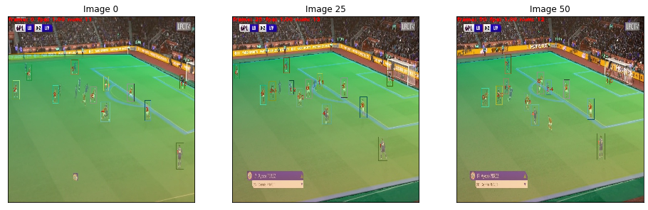
Let’s check the same images as before but with the tracking informations:
imgs_ordered = []
for i in range(0,51):
    path = 'test_outputs/test_' + '{:05d}'.format(i) + '.jpg'
    imgs_ordered.append(path)

img_list = []
for path in imgs_ordered:
    if path.endswith('.jpg'):
        image = cv2.imread(path)
        image = cv2.cvtColor(image, cv2.COLOR_BGR2RGB)
        img_list.append(image)

image_0,image_25,image_50 = img_list[0],img_list[25],img_list[50]
print("Image shape: {}".format(image_0.shape))
visualize(image_0=image_0,
            image_25=image_25,
            image_50=image_50)
You can also easily create a movie of the tracking data, and display it:
import imageio
import progressbar
with imageio.get_writer('test_outputs/movie.mp4', mode='I',fps=20) as writer:
    for i in progressbar.progressbar(range(0,51)):
        filename = 'test_outputs/test_{:05d}.jpg'.format(i)
        image = imageio.imread(filename)
        writer.append_data(image)
100% (51 of 51) |########################| Elapsed Time: 0:00:00 Time: 0:00:00
Process trajectories
We now have raw trajectories that we need to process. Fist, you can do several operations to ensure that the trajectories are functional:
- Delete an id at a specific frame
- Delete an id from every frame
- Merge two ids
- Add an id at a given frame
These operations are simple to do with some of our functions from narya.utils.tracker:
def _remove_coords(traj, ids, frame):
    """Remove the x,y coordinates of an id at a given frame
    Arguments:
        traj: Dict mapping each id to a list of trajectory
        ids: the id to target
        frame: int, the frame we want to remove
    Returns:
        traj: Dict mapping each id to a list of trajectory
    Raises:
    """

def _remove_ids(traj, list_ids):
    """Remove ids from a trajectory
    Arguments:
        traj: Dict mapping each id to a list of trajectory
        list_ids: List of id
    Returns:
        traj: Dict mapping each id to a list of trajectory
    Raises:
    """

def add_entity(traj, entity_id, entity_traj):
    """Adds a new id with a trajectory
    Arguments:
        traj: Dict mapping each id to a list of trajectory
        entity_id: the id to add
        entity_traj: the trajectory linked to entity_id we want to add
    Returns:
        traj: Dict mapping each id to a list of trajectory
    Raises:
    """

def add_entity_coords(traj, entity_id, entity_traj, max_frame):
    """Add some coordinates to the trajectory of a given id
    Arguments:
        traj: Dict mapping each id to a list of trajectory
        entity_id: the id to target
        entity_traj: List of (x,y,frame) to add to the trajectory of entity_id
        max_frame: int, the maximum number of frame in trajectories
    Returns:
        traj: Dict mapping each id to a list of trajectory
    Raises:
    """


def merge_id(traj, list_ids_frame):
    """Merge trajectories of different ids.
    e.g.: (10,0,110),(12,110,300) will merge the trajectory of 10 between frame 0 and 110 to the
        trajectory of 12 between frame 110 and 300.
    Arguments:
        traj: Dict mapping each id to a list of trajectory
        list_ids_frame: List of (id,frame_start,frame_end)
    Returns:
        traj: Dict mapping each id to a list of trajectory
    Raises:
    """

def merge_2_trajectories(traj1, traj2, id_mapper, max_frame_traj1):
    """Merge 2 dict of trajectories, if you want to merge the results of 2 tracking
    Arguments:
        traj1: Dict mapping each id to a list of trajectory
        traj2: Dict mapping each id to a list of trajectory
        id_mapper: A dict mapping each id in traj1 to id in traj2
        max_frame_traj1: Maximum number of frame in the first trajectory
    Returns:
        traj1: Dict mapping each id to a list of trajectory
    Raises:
    """
Here, let’s assume we don’t have to perform any operations, and directly process our trajectories into a Pandas Dataframe.
First, we can save our raw trajectory with
import json

with open('trajectories.json', 'w') as fp:
    json.dump(trajectories, fp)
Let’s start by padding our trajectories with np.nan and building a dict. for our dataframe:
import json

with open('trajectories.json') as json_file:
    trajectories = json.load(json_file)
from narya.utils.tracker import build_df_per_id

df_per_id = build_df_per_id(trajectories)
We now fill the missing values, and apply a filter to smooth the trajectories:
from narya.utils.tracker import fill_nan_trajectories

df_per_id = fill_nan_trajectories(df_per_id,5)
from narya.utils.tracker import get_full_results

df = get_full_results(df_per_id)
Trajectory Dataframe
We now have access to a dataframe with for each id, for each frame, the 2D coordinates of the entity.
df.head()
| id | x | y | |
|---|---|---|---|
| frame | |||
| 1 | 1 | 78.251729 | 10.133520 |
| 2 | 1 | 78.262442 | 10.138342 |
| 3 | 1 | 78.308051 | 10.483425 |
| 4 | 1 | 78.356691 | 10.792084 |
| 5 | 1 | 78.379051 | 10.967897 |
Finally, this you can save this dataframe using df.to_csv('results_df.csv')
EDG
Now that we have some tracking data, it is time to evaluate them.
Theoretical framework
We assume $s_t \in \mathcal{S}$ is the state of the game at time $t$. It may be the positions of each player and the ball for example. Given an action $a \in \mathcal{A}$ (\eg a pass, a shot,etc), and a state $s’ \in \mathcal{S}$, we note $\mathbb{P} \colon \mathcal{S} \times \mathcal{A} \times \mathcal{S} \to [0,1]$ the probability $\mathbb{P} (s’ \vert s, a)$ of getting to state $s’$ from $s$ following action $a$. % Applying actions over $K$ time steps yields a trajectory of states and actions, $\tau ^{t_{0:K}} = \big(s_{t_0},a_{t_0}, … ,s_{t_K},a_{t_K} \big)$. We denote $r_t$ the reward given going from $s_t$ to $s_{t+1}$ (\eg $+1$ if the team scores a goal). More importantly, the cumulative discounted reward along $\tau ^{t_{0:K}}$ is defined as:
\[R(\tau ^{t_{0:K}}) = \sum_{n=0}^{K} \gamma^{n} r_{t_n}\]where $\gamma \in \left[0,1\right]$ is a discount factor, smoothing the impact of temporally distant rewards.
A policy, $\pi _{\theta}$, chooses the action at any given state, whose parameters, $\theta$, can be optimized for some training objectives (such as maximizing $R$). Here, a good policy would be a policy representing the team we want to analyze in the right manner. The \textit{Expected Discounted Goal} (EDG), or more generally, the state value function, is defined as:
\[V^\pi (s) = \underset{\tau \sim \pi}{\mathbb{E}} \big[ R(\tau) \vert s \big]\]It represents the discounted expected number of goals the team will score (or concede) from a particular state. To build such a good policy, one can define an objective function based on the cumulative discounted reward:
\[J(\theta) = \underset{\tau \sim \pi_\theta}{\mathbb{E}} \big[ R(\tau) \big]\]and seek the optimal parametrization $\theta ^*$ that maximize $J(\theta)$:
\[\theta^* = \arg \max_\theta \mathbb{E} \big[ R(\tau) \big]\]To that end, we can compute the gradient of such cost function\footnote{Using a log probability trick, we can show that we have the following equality: $\nabla_\theta J(\theta) = \underset{\tau \sim \pi_\theta}{\mathbb{E}} \left[ \sum_{t=0}^T \nabla_\theta \log \left( \pi_\theta (a_t \vert s_t) \right) R(\tau) \right]$} $\nabla_\theta J(\theta)$ to update our parameters with $\theta \leftarrow \theta + \lambda \nabla_\theta J(\theta)$. In our case, the evaluation of $V^\pi$ and $\pi_\theta$ is done using Neural Networks, and $\theta$ represents the weights of such networks. At inference, our model will take the state of the game as input, and will output the estimation of the EDG.
Implementation
Our EDG agent was implemented using the Google Football library. We trained our agent against bots and against itself until it became strong enough. Such an agent can be seen on this youtube video.
Let’s start by importing some libraries:
Notes: Google Football is not compatible with Tensorflow 2 yet. We have to downgrade it to use our agent.
!pip3 install --user tensorflow==1.15.*
!pip3 install --user tensorflow-probability==0.5.0
!pip3 install --user dm-sonnet==1.*
from matplotlib import pyplot as plt
import pandas as pd
import numpy as np
Like the tracking models, our agent can easily be created:
from narya.analytics.edg_agent import AgentValue
import tensorflow as tf

WEIGHTS_PATH = (
    "https://storage.googleapis.com/narya-bucket-1/models/11_vs_11_selfplay_last"
)
WEIGHTS_NAME = "11_vs_11_selfplay_last"
WEIGHTS_TOTAR = False

checkpoints = tf.keras.utils.get_file(
                WEIGHTS_NAME, WEIGHTS_PATH, WEIGHTS_TOTAR,
            )

agent = AgentValue(checkpoints = checkpoints)
Loading and processing tracking data
First, we need to process our tracking data into a Google Football format. We built a few functions to do this.
Let’s load some tracking data from Liverpool:
data = pd.read_csv('liverpool_2019.csv', index_col=('play', 'frame'))
data['edgecolor'] = data['edgecolor'].fillna(0)
data.tail()
| Unnamed: 0 | bgcolor | dx | dy | edgecolor | player | player_num | team | x | y | z | ||
|---|---|---|---|---|---|---|---|---|---|---|---|---|
| play | frame | |||||||||||
| Leicester 0 - [3] Liverpool | 120 | 2745 | blue | 0.0 | 0.0 | white | 10267 | NaN | defense | 98.724826 | 53.720353 | 0.0 |
| 121 | 2746 | blue | 0.0 | 0.0 | white | 10267 | NaN | defense | 98.724826 | 53.720353 | 0.0 | |
| 122 | 2747 | blue | 0.0 | 0.0 | white | 10267 | NaN | defense | 98.724826 | 53.720353 | 0.0 | |
| 123 | 2748 | blue | 0.0 | 0.0 | white | 10267 | NaN | defense | 98.724826 | 53.720353 | 0.0 | |
| 124 | 2749 | blue | 0.0 | 0.0 | white | 10267 | NaN | defense | 98.724826 | 53.720353 | 0.0 |
Let’s process them to add some features:
from narya.utils.google_football_utils import _add_ball_coordinates, _add_possession
data = data.rename(columns={'edgecolor':'id'})
data_test = _add_ball_coordinates(data,id_ball=0)
data_test = _add_possession(data_test)
data_test = data_test.rename(columns={'id':'edgecolor'})
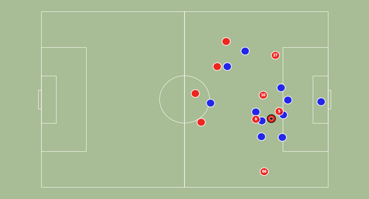
We can chose one game, and display the first frame:
play =  'Leicester 0 - [3] Liverpool'
df = data_test[data_test['play'] == play]
df = df.set_index('frame')
df['bgcolor'] = df['bgcolor'].fillna('black')
df.tail()
| bgcolor | dx | dy | edgecolor | player | player_num | team | x | y | z | ball_x | ball_y | ball_z | play | possession | |
|---|---|---|---|---|---|---|---|---|---|---|---|---|---|---|---|
| frame | |||||||||||||||
| 120 | blue | 0 | 0 | white | 10267 | NaN | defense | 98.7248 | 53.7204 | 0 | 100.68 | 44.958 | 0 | Leicester 0 - [3] Liverpool | False |
| 121 | blue | 0 | 0 | white | 10267 | NaN | defense | 98.7248 | 53.7204 | 0 | 100.68 | 44.958 | 0 | Leicester 0 - [3] Liverpool | False |
| 122 | blue | 0 | 0 | white | 10267 | NaN | defense | 98.7248 | 53.7204 | 0 | 100.68 | 44.958 | 0 | Leicester 0 - [3] Liverpool | False |
| 123 | blue | 0 | 0 | white | 10267 | NaN | defense | 98.7248 | 53.7204 | 0 | 100.68 | 44.958 | 0 | Leicester 0 - [3] Liverpool | False |
| 124 | blue | 0 | 0 | white | 10267 | NaN | defense | 98.7248 | 53.7204 | 0 | 100.68 | 44.958 | 0 | Leicester 0 - [3] Liverpool | False |
from narya.utils.vizualization import draw_frame

fig, ax, dfFrame = draw_frame(df,t=0,add_vector = False,fps=20)
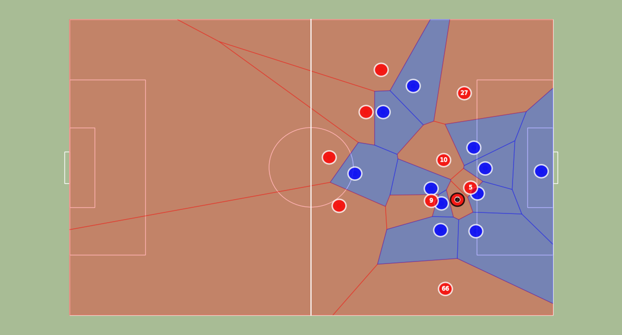
We can also add a Voronoi Diagram and velocity vectors on our field:
from narya.utils.vizualization import add_voronoi_to_fig

fig, ax, dfFrame = draw_frame(df,t=0,fps=20)
fig, ax, dfFrame = add_voronoi_to_fig(fig, ax, dfFrame)
Google Format
We now have to change our data into a google format. To do so, we need to change:
- the Ball positions and velocity
- the Players positions and velocity
- Who owns the ball, and what team he is in
And transfer the coordinates in a different representation.
from narya.utils.google_football_utils import _save_data, _build_obs_stacked
,
data_google = _save_data(df,'test_temo.dump')
observations = {
    'frame_count':[],
    'obs':[],
    'obs_count':[],
    'value':[]
}

for i in range(len(data_google)):
    obs,obs_count = _build_obs_stacked(data_google,i)
    observations['frame_count'].append(i)
    observations['obs'].append(obs)
    observations['obs_count'].append(obs_count)
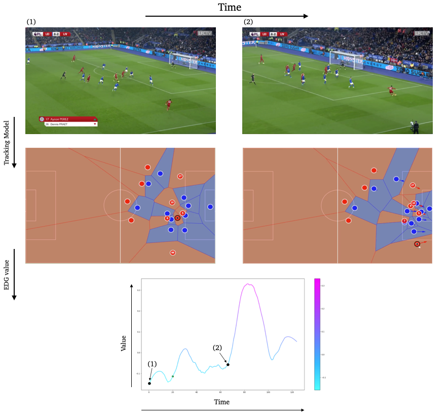
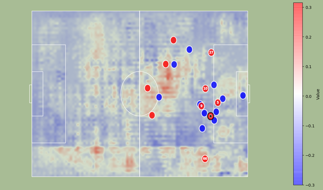
We can now plot an EDG map at $t=1$. It represents the location with the most potential on the field.
map_value = agent.get_edg_map(observations['obs'][20],observations['obs_count'][20],79,57,entity = 'ball')
from narya.utils.vizualization import add_edg_to_fig

fig, ax, dfFrame = draw_frame(df, t=1)
fig, ax, edg_map = add_edg_to_fig(fig, ax, map_value)
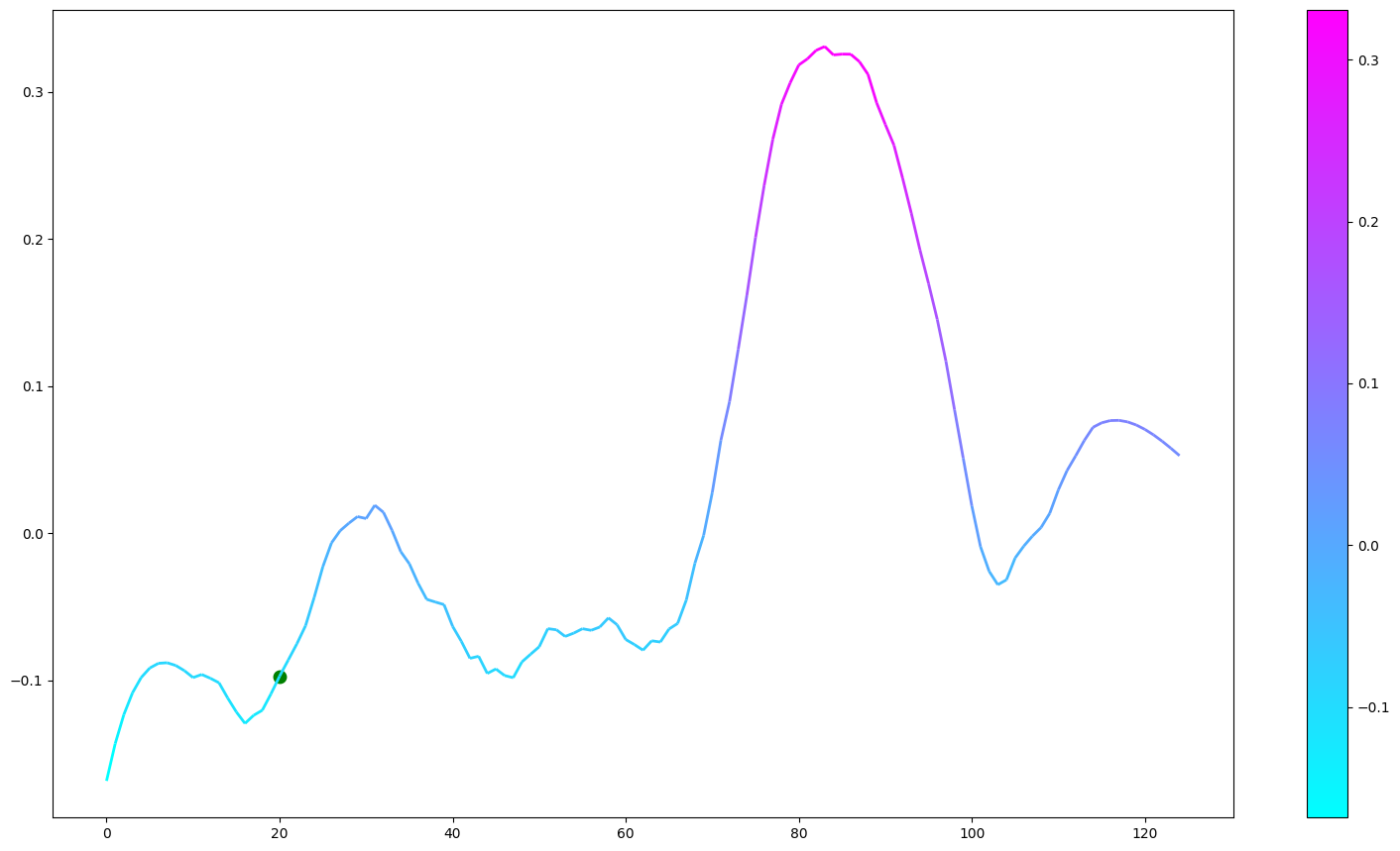
You can also plot the EDG value over time:
from narya.utils.vizualization import draw_line

for indx,obs in enumerate(observations['obs']):
    value = agent.get_value([obs])
    observations['value'].append(value)
df_dict = {
    'frame_count':observations['frame_count'],
    'value':observations['value']
}
df_ = pd.DataFrame(df_dict)
fig, ax = draw_line(df_,1,20, smooth=True)
Training and datasets
Finally, we also release our datasets and models.
Datasets
Links:
| Model | Description | Link |
|---|---|---|
| 11_vs_11_selfplay_last | EDG agent | https://storage.googleapis.com/narya-bucket-1/models/11_vs_11_selfplay_last |
| deep_homo_model.h5 | Direct Homography estimation Architecture | https://storage.googleapis.com/narya-bucket-1/models/deep_homo_model.h5 |
| deep_homo_model_1.h5 | Direct Homography estimation Weights | https://storage.googleapis.com/narya-bucket-1/models/deep_homo_model_1.h5 |
| keypoint_detector.h5 | Keypoints detection Weights | https://storage.googleapis.com/narya-bucket-1/models/keypoint_detector.h5 |
| player_reid.pth | Player Embedding Weights | https://storage.googleapis.com/narya-bucket-1/models/player_reid.pth |
| player_tracker.params | Player & Ball detection Weights | https://storage.googleapis.com/narya-bucket-1/models/player_tracker.params |
The datasets can be downloaded at:
| Dataset | Description | Link |
|---|---|---|
| homography_dataset.zip | Homography Dataset (image,homography) | https://storage.googleapis.com/narya-bucket-1/dataset/homography_dataset.zip |
| keypoints_dataset.zip | Keypoint Dataset (image,list of mask) | https://storage.googleapis.com/narya-bucket-1/dataset/keypoints_dataset.zip |
| tracking_dataset.zip | Tracking Dataset in VOC format (image, bounding boxes for players/ball) | https://storage.googleapis.com/narya-bucket-1/dataset/tracking_dataset.zip |
Overview
Homography Dataset: The homography dataset is made of pair of images,matrix in a .jpg,.npy format. The matrix is the homography associated with the image. They are normalized, meaning that homography[2,2] == 1.
Keypoints Dataset: We give here pair of images,xml file. The .xml files are made of the coordinates of each available keypoints on the image. We built utils function to read these files, and do so automaticaly in our Dataset class.
Tracking Dataset: Pair of images,xml files in a VOC format.
Training
Finally, we give here a quick tour of our training scripts.
We start by creating a model:
full_model = KeypointDetectorModel(
    backbone=opt.backbone, num_classes=29, input_shape=(320, 320),
)

if opt.weights is not None:
    full_model.load_weights(opt.weights)
We then create a loss function and an optimizer:
# define optomizer
optim = keras.optimizers.Adam(opt.lr)
# define loss function
dice_loss = sm.losses.DiceLoss()
focal_loss = sm.losses.CategoricalFocalLoss()
total_loss = dice_loss + (1 * focal_loss)

metrics = [sm.metrics.IOUScore(threshold=0.5), sm.metrics.FScore(threshold=0.5)]

# compile keras model with defined optimozer, loss and metrics
model.compile(optim, total_loss, metrics)

callbacks = [
    keras.callbacks.ModelCheckpoint(
        name_model, save_weights_only=True, save_best_only=True, mode="min"
    ),
    keras.callbacks.ReduceLROnPlateau(
        patience=10, verbose=1, cooldown=10, min_lr=0.00000001
    ),
]

model.summary()
We can easily build a Dataset and a Dataloader (handling batches):
x_train_dir = os.path.join(opt.data_dir, opt.x_train_dir)
kp_train_dir = os.path.join(opt.data_dir, opt.y_train_dir)
x_test_dir = os.path.join(opt.data_dir, opt.x_test_dir)
kp_test_dir = os.path.join(opt.data_dir, opt.y_test_dir)

full_dataset = KeyPointDatasetBuilder(
    img_train_dir=x_train_dir,
    img_test_dir=x_test_dir,
    mask_train_dir=kp_train_dir,
    mask_test_dir=kp_test_dir,
    batch_size=opt.batch_size,
    preprocess_input=preprocessing_fn,
)

train_dataloader, valid_dataloader = full_dataset._get_dataloader()
Finally, easily launch a training with:
model.fit_generator(
    train_dataloader,
    steps_per_epoch=len(train_dataloader),
    epochs=opt.epochs,
    callbacks=callbacks,
    validation_data=valid_dataloader,
    validation_steps=len(valid_dataloader),
)