A review on Deep Reinforcement Learning for Fluid Mechanics
I now work at Flaneer, feel free to reach out if you are interested!
When I started an Internship at the CEMEF, I’ve already worked with both Deep Reinforcement Learning (DRL) and Fluid Mechanics, but never used one with the other. I knew that several people already went down that lane, some where even currently working at the CEMEF when I arrived. However, I (and my tutor Elie Hachem) still had several questions/goals on my mind :
- How was DRL applied to Fluid Mechanics?
- To improve in both subject, I wanted to try a test case on my own;
- How could we code something as general as possible?
The results of these questions are available here, with the help of a fantastic team.
Applications of DRL to Fluid mechanics
Several Fluid Mechanics problems have already been tackled with the help of DRL. They always (mostly) follow the same pattern, using DRL tools on one side (such as Gym, Tensorforce or stables-baselines, etc) and Computational Fluid Dynamics (CFD) on the other (Fenics, Openfoam, etc).
Currently, most of the reviewed cases always consider objects (a cylinder, a square, a fish, etc.) in a 2D/3D fluid. The DRL agent will then be able to perform several tasks :
- Move the object
- Change the geometry or size of the object
- Change the fluid directly
This agent can perform these tasks at two key moments : (i) when the experiment is done, and you want to start a new one, (ii) during the experiment (i.e., during the CFD time). One is about direct optimization; the other one is about continuous control. A few examples can be seen below :
and even this video. (which is pretty amazing)
My own test case
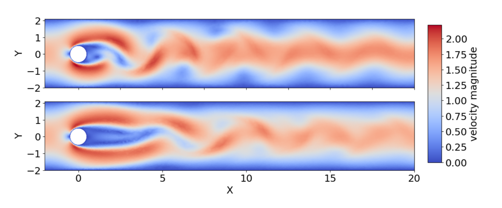
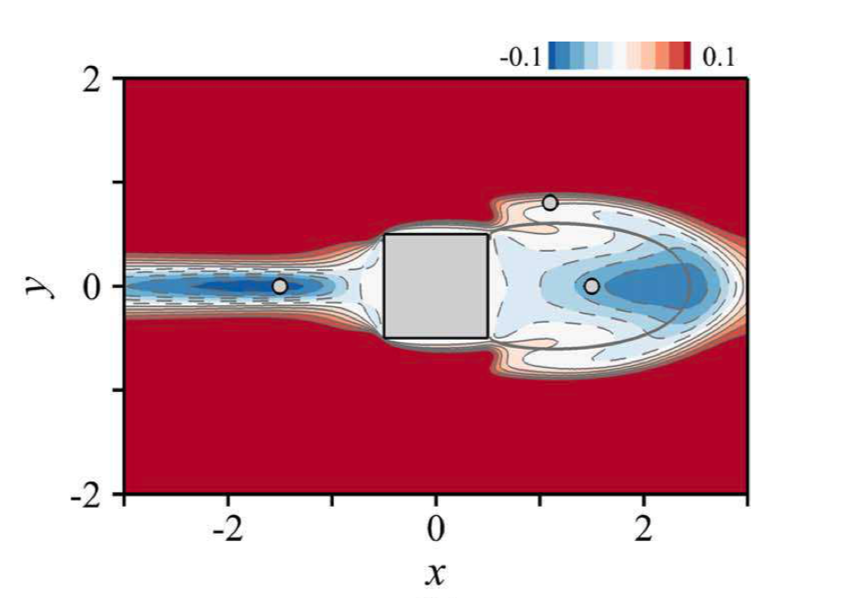
In order to dive deeper into the subject, I wanted to try a test case on my own (with the help of Jonathan Viquerat at the beginning though). We took inspiration from this paper and considered a simple case: a laminar flow past a square. Now, it is convenient to compute the drag of this square (in this very set-up).
However, the question asked by the paper was: if we add a tiny cylinder, somewhere close to the square, could we be able to reduce the total drag of both the square and the small cylinder?
The answer is yes, and the result is shown below:
Now, of course solving this case with DRL was interesting, but I wanted to see if more was possible (since the case was already settled technically). Several ideas were possible (thanks to discussions with peoples from the CEMEF and the review I did previously) :
- Was there any difference between direct optimization and continuous control?
- Was the use of an autoencoder easy?
- Was Transfer Learning possible, and performant?
- Could we make a code as clear as possible?
Regarding the first point, I found no particular difference between direct optimization and continuous control. Both agents converge and find almost the same optimal final positions.
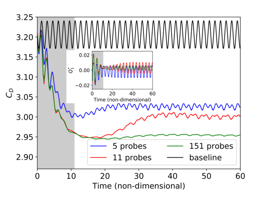
I used an autoencoder but had no time no compare results with and without it. I do have to explain why an autoencoder could be of any help here. The agent needs observations, and when dealing with fluid mechanics, the fluid characteristics are significant observations.
However, they can be of very high dimensions (more than 10,000). The Neural Network (NN) we would deal with would then be incredibly vast. In order to surpass this issue, an autoencoder could be used to extract simple features from high-dimensional fluid fields. It does seem like using as many fluid features as possible (which is possible with the autoencoder) is the best thing to do:
In total, I trained six agents, as shown below :
| Agent | Reynolds Number - Re | Goal | Details |
|---|---|---|---|
| Agent 3.2 | Re=100 | Direct optimization | Transfer learning from Agent 1.2 |
| Agent 1.1 | Re=10 | Continuous control | Trained from scratch |
| Agent 1.2 | Re=10 | Direct optimization | Trained from scratch |
| Agent 2.1 | Re=40 | Continuous control | Transfer learning from Agent 1.1 |
| Agent 2.2 | Re=40 | Direct optimization | Transfer learning from Agent 1.2 |
| Agent 3.1 | Re=100 | Continuous control | Transfer learning from Agent 1.1 |
As you can see, I used transfer learning and obtained excellent results from it: the agent was learning from 5 to 10 times faster than the agent trained from scratch. This is an exciting feature in general, but especially for Fluid Dynamics, where CFD is computationally expensive.
A DRL-fluid mechanics library?
At the beginning, my goal was to find out if such a library could be built (in a reasonable amount of time). During the creation of my test case, I realized the biggest issue with such a library was coming from the CFD solver: not only no one is using the same, but they all are pretty different.
For my test case, I based my code on Fenics, an easy-to-use solver (and super convenient since you can use it directly in Python). The code is available here. It is supposed to be as clear and re-usable as possible. It is based on Gym and stable-baselines.
I used Gym to build custom environment, always following the same pattern :
class FluidMechanicsEnv_(gym.Env):
    metadata = {'render.modes': ['human']}
    def __init__(self,
                    **kwargs):
        ...
        self.problem = self._build_problem()
        self.reward_range = (-1,1)
        self.observation_space = spaces.Box(low=np.array([]), high=np.array([]), dtype=np.float16)
        self.action_space = spaces.Box(low=np.array([]), high=np.array([]), dtype=np.float16)
    def _build_problem(self,main_drag):
        ...
        return problem
    def _next_observation(self):
        ...
    def step(self, action):
        ...
        return obs, reward, done, {}
    def reset(self):
        ...
With stable-baselines, I used their DRL algorithms implementations, and finally, as I said earlier, I used Fenics to build my test case using custom class that I hope will be re-used for other test cases. They use three main class: Channel, Obstacles, and Problem :
Channel :
Basically, this is the box you want your experiment to take place in. You only define it by giving the lower and upper corner of the box.
class Channel:

    """
    Object computing where our problem will take place.
    At the moment, we restraint ourself to the easier domain possible : a rectangle.
    :min_bounds:    (tuple (x_min,y_min))   The lower corner of the domain
    :max_bounds:    (tuple (x_max,y_max))   The upper corner of the domain
    :Channel:       (Channel)               Where the simulation will take place
    """
    def __init__(self,
                min_bounds,
                max_bounds,
                type='Rectangle'):
Obstacles :
This is the objects you want to add to the previously seen box. If you only want to use Fenics, you can only easily add squares, circles, or polygons. However, if you want to add much more complex shapes and mesh, you can use the Mesh function from Fenics.
class Obstacles:

    """
    These are the obstacles we will add to our domain.
    You can add as much as you want.
    At the moment, we only take care of squares and circles and polygons
    :size_obstacles:    (int)           The amount of obstacle you wanna add
    :coords:            (python list)   List of tuples, according to 'fenics_utils.py : add_obstacle'
    :Obstacles:         (Obstacles)     An Obstacles object containing every shape we wanna add to our domain
    """


    def __init__(self,
                size_obstacles=0,
                coords = []):
Problem :
This is where everything is taking place: setting up the box, placing the several objects, defining the boundary conditions, etc.
class Problem:

    def __init__(self,
                min_bounds,
                max_bounds,
                import_mesh_path = None,
                types='Rectangle',
                size_obstacles=0,
                coords_obstacle = [],
                size_mesh = 64,
                cfl=5,
                final_time=20,
                meshname='mesh_',
                filename='img_',
                **kwargs):

        """
        We build here a problem Object, that is to say our simulation.
        :min_bounds:                (tuple      (x_min,y_min)) The lower corner of the domain
        :max_bounds:                (tuple      (x_max,y_max)) The upper corner of the domain
        :import:import_mesh_path:   (String)    If you want to import a problem from a mesh, and not built it with mshr
        :types:                     (String)    Forced to Rectangle at the moment
        :size_obstacle:             (int)       The amount of shape you wanna add to your domain
        :coords_obstacle:           (tuple)     the parameters for the shape creation
        :size_mesh:                 (int)       Size of the mesh you wanna create
        :cfl:                       (int)
        :final_time:                (int)       Length of your simulation
        :mesh_name:                 (String)    Name of the file you wanna save your mesh in
        :filename:                  (String)    Name of the file you wanna save the imgs in
        """
However, this is not getting even close to a true DRL-fluid mechanics library, the issue being Fenics. While being very easy to use, it is a slow solver, and it would be impracticable to use it for a challenging problem. This is why, with other people working at the CEMEF, the goal is to build this library, linking DRL with other CFD libraries, most of them being C++ based.
References
-
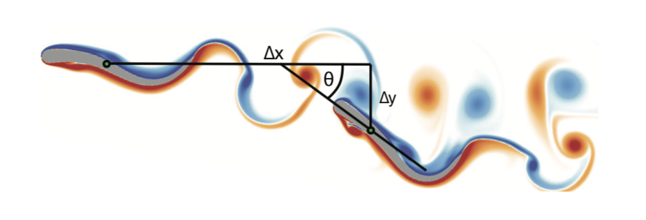
Synchronisation through learning for two self-propelled swimmers - Novati et al. (2017)
-
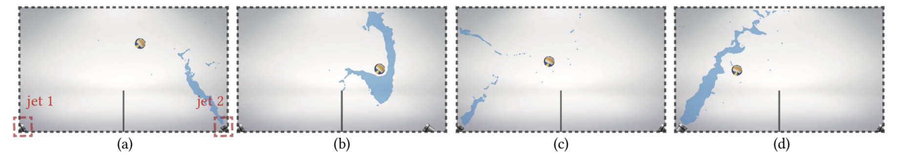
fluid directed rigid body control using deep reinforcement learning - Ma et al. (2018)
-
A review on Deep Reinforcement Learning for Fluid Mechanics - Garnier et al. (2019)